

Week 3: Free Energy and Shannon Entropy
[jupyter][google colab][reveal][edit]
Abstract:
Homework from Weeks 1–2, then the heat thread from quantity toward free energy: Black, Carnot, Rumford, the air thermometer, Thomson’s 1848 mill-scale, Joule. After the break, Helmholtz \(F=U-TS\) on the board; Clausius after that. Shannon, Jaynes and Wiener appear as a close preview. The entropy game and MacKay’s weighing problem were named and not reached; they now open Week 4 after Quiz 2. Shannon axioms, HMC, \(Z\), KL and Schottky live in _lamd/parking.md.
No class test today. Next week there is a class test, even if the webpage said otherwise on 27 October. Laptops away; notes by hand. The slot is 10:05–11:55 (110 minutes, not 120). As taught, the homework debrief ran about twenty-four minutes, then the heat thread as far as Joule before the break. Helmholtz was the LO1 payload after the break, on the visualiser, before the Clausius slides. Maxwell–Boltzmann and Gibbs were pointers, not the planned decks. Shannon / Jaynes / Wiener were a close preview. The entropy game and MacKay’s weighing problem were not given; they now open Week 4 after Quiz 2. Shannon axioms, HMC, \(Z\), KL, Schottky and finite-time live in _lamd/parking.md.
This Session
Time plan (as delivered 27 October 2026). Clocks from the Panopto SRT (recording 00:00 ≈ 10:00). The slot is 10:05–11:55 (110 minutes, not 120). Speech from 10:04; this session ran to about 11:58. Helmholtz on the board is the LO1 payload. Shannon / Jaynes / Wiener and Maxwell’s demon as coarse-graining are previews of later weeks. MacKay / entropy game stay in the file; they were not given.
| Clock | Block |
|---|---|
| 10:04–10:06 | Laptops away |
| 10:06–10:09 | This session: heat story, Helmholtz, MacKay if time |
| 10:09–10:23 | Quiz 1 debrief (mean \(8.2/10\); gremlin; energy as score; coldness) |
| 10:23–10:32 | Worksheet 1 (mean \(12.2\); rat-hole; see-saw) |
| 10:32–10:33 | Worksheet 2 already out; quiz 2 next week |
| 10:33–10:37 | The story of the lecture |
| 10:37–10:45 | Joseph Black: latent heat; Watt; calorimeter |
| 10:45–10:53 | Carnot: mill, caloric, Clapeyron, cholera |
| 10:53–10:56 | Rumford: inexhaustible heat |
| 10:56–11:01 | Air thermometer; Thomson 1848 |
| 11:01–11:05 | Joule; the contradiction; Clausius after the break |
| 11:05–11:13 | Break |
| 11:13–11:17 | Pens; Cavendish / royal-commission aside |
| 11:17–11:48 | Helmholtz on the visualiser; questions (\(T\)–\(S\) square; four-stroke) |
| 11:48–11:54 | Clausius; Maxwell–Boltzmann pointer |
| 11:54–11:58 | Preview: Shannon / Jaynes / Wiener; class test next week |
The include order below is still Black \(\to\) \(\to\) Helmholtz. As taught, Helmholtz was boarded after Joule and before the Clausius slides. Protect Helmholtz. The information game, MacKay and grouping now open Week 4 after Quiz 2. Shannon / HMC / Schottky live in _lamd/parking.md.
Homework from Weeks 1–2
No quiz today — the class test is next week, even if the webpage said otherwise on 27 October. Feedback on Worksheet 1 and Quiz 1, then the heat thread. Comments go by email; marks do not appear on these slides, and names do not either. The numbers below are cohort figures from the marked scripts. Laptops away for the rest of the course: notes by hand.
Quiz 1
The paper was ten items on the Week 1 probability review and the energy / Boltzmann seeds. Matching and the two-state \(Z\) were essentially clean. Two multi-select items were where most marks were lost.
Named distributions, the multinomial, curiosity-then-skepticism, the two-state partition function, and Bayes needing likelihoods and priors were mostly all got correct (well done). Boltzmann weights and the sum/product rules had a smaller tail. The two ideas worth looking at again for some are demons and gremlins and energy-as-score.
Week 1 put both figures on the table, and the quiz asked you to keep them apart. A majority of papers mixed them. Maxwell’s demon is a sorting intelligence that appears to drop the entropy of a gas. Laplace’s demon is a predictive intelligence. Laplace’s gremlin (Neil’s invention) is about the practical impossibility of knowing the positions and momenta of every molecule as well as the rules and then doing the resulting computations. The gremlin is why we need a statistical description at all. That will also be the bridge into today’s free-energy to entropy story. The word itself is from aircraft: in the First World War they blamed gremlins for things going wrong in the planes. Two demons, one gremlin.
The other expensive item asked which of the Week 1 energy remarks actually hold for machine learning. Lower energy corresponds to a more preferred, more probable state. Quadratic loss and cross-entropy can be written as energy-like scores. What does not follow is that every use of the word energy in an ML paper is a valid thermodynamic internal energy, or that a heat bath has been specified. We will cover the relationship today. \(\beta\) is inverse temperature, or coldness; Cole Palmer has a high \(\beta\). From an entropic perspective coldness is the more natural parameter than \(T\).
Worksheet 1
Thirteen dialogues, marked 5 curiosity / 5 skepticism / 5 reflection. Cohort means: curiosity \(4.4\), skepticism \(4.2\), reflection \(3.9\) on the twelve reflections present. The work was strong. The comments clustered on a few habits I want in the room before Worksheet 2, which is already out and due at the start of lecture 4.
Several dialogues pulled in material I had not put in the brief — IAS, a Masters thesis, interviews, Schrödinger, the bandwagon paper, Markov chains and Kolmogorov complexity, the H-theorem versus Gibbs confusion, Jaynes on the observer. That is curiosity doing what it is for. The recurring gap was not ignorance of Shannon’s footnote. It was how to keep a ten-turn chat moving after the first successful challenge.
I used “see-saw” in the comments for a pattern that showed up across models: you contradict, it caves, you have won a turn and lost a thread. The Grasshopper in Suits does not fold when Skepticus objects. Current chat models are trained to satisfy. Intellectual judo — stating the point of agreement in your own words, or framing the objection as a possible misunderstanding — kept the better dialogues in motion. Long, specific prompts also helped; they give the model less room to treat the last user turn as a verdict to submit to.
A few dialogues got a precise definition and then spent the remaining turns litigating it. Push-back is the skepticism mark, but remaining in the same hole for five turns is rat-holing! The dialogues that recovered did something simple: after pushing for two or three exchanges they changed the question, taking what had been established as a premise. Model choice also mattered. Gemini Flash, in several scripts, gave shorter answers that were easier to steer than a larger, more fluent model. Claude models were a little too verbose which made it easy to point out a flaw and end up see-sawing. DeepSeek, in one case, had to be led by the hand. The reflection is the place to say why you stayed with the model you stayed with — several reflections missed that.
This was the probe I kept writing in the comments. If Shannon’s \(H\) is “entropy as uncertainty,” someone in physics must already have treated entropy that way, or Shannon (and Wiener) did it independently. It is not in Clausius. It is in the Boltzmann–Gibbs statistical reading, and Wiener is explicit that his information comes from a Gibbsian theory of ignorance. Whether Wiener and Shannon had that conversation before 1948 is a historical question the models will fluently invent. Primary sources still beat that attempt at fluency. Shannon footnotes Tolman; he credits Wiener in another footnote; the von Neumann cocktail party seems to be later folklore. Worksheet 2 asks a sharper version of the same issue: once the name is granted, is \(H\) the same mathematical object as \(S\), or a metaphor?
Worksheet 2 was released in Week 2. The brief is in the notes from that session and on the course site. Ten turns, one continuous conversation, one declared model; handwritten reflection on the proforma. The subject is no longer why Shannon named the quantity, but what the naming claims. If the model says identity of form, ask what must be true of the sample space. If it says metaphor, ask what the metaphor licenses. Reflection should include how the inquiry habit has changed since Worksheet 1 — that was the weakest of the three marks this round, and it is explicitly in the W2 rubric.
From Heat to Helmholtz
Week 1 seeded the occupation \(p_i \propto e^{-\beta E_i}\). Worksheet 1 told us Clausius did not make entropy a measure of uncertainty. The lecture is the heat thread that gets us to Helmholtz: Black, Carnot, Rumford, the air thermometer, Thomson’s 1848 mill-scale, Joule — then, as taught, the board work on \(F=U-TS\) with \(U=\left\langle E\right\rangle\), and Clausius after that. Maxwell–Boltzmann and Gibbs remain in the file after Clausius. The entropy game and MacKay’s weighing problem come after that story; they were not reached on 27 October and now open Week 4 after Quiz 2. Shannon axioms live in _lamd/parking.md.
From a stationary distribution with given energy we will write the Gibbs distribution, \[ p_i = \frac{e^{-\beta E_i}}{Z} \quad Z = \sum_i e^{-\beta E_i}. \] The destination of the thread is \[ U = F + TS \] where \(U=\left\langle E\right\rangle\) is inner energy, \(F\) is Helmholtz free energy, \(T\) is temperature and \(S\) is physical entropy. Physical entropy is the dimensionless functional \(H=-\sum_i p_i\log p_i\) converted into joules per degree by Boltzmann’s constant, \(S=k_B H\). Helmholtz wrote \(A=U-TS\) (\(A\) for Arbeit); we use \(F\) for the same quantity because week 5 needs \(A(\boldsymbol{\theta})\) for the log-partition.
Information, energy and intelligence course notebook setup
We install some bespoke code for creating and saving plots as well as loading data sets.
import importlib.utilcmd = install_command('pods')%system {cmd}cmd = install_command('notutils')%system {cmd}cmd = install_command('mlai')%system {cmd}Joseph Black and Heat as a Quantity
Before heat was understood as a property, it was understood as a quantity. For Clausius, entropy was not yet a measure of uncertainty, but to try and understand what he was measuring we need to go back to heat. For our purposes the intellectual thread starts with Joseph Black (1728–1799) who is responsible for making heat a quantity you can measure, mix and even hide. This notion of heat as a measurable is different from the notion of temperature as a measurable.
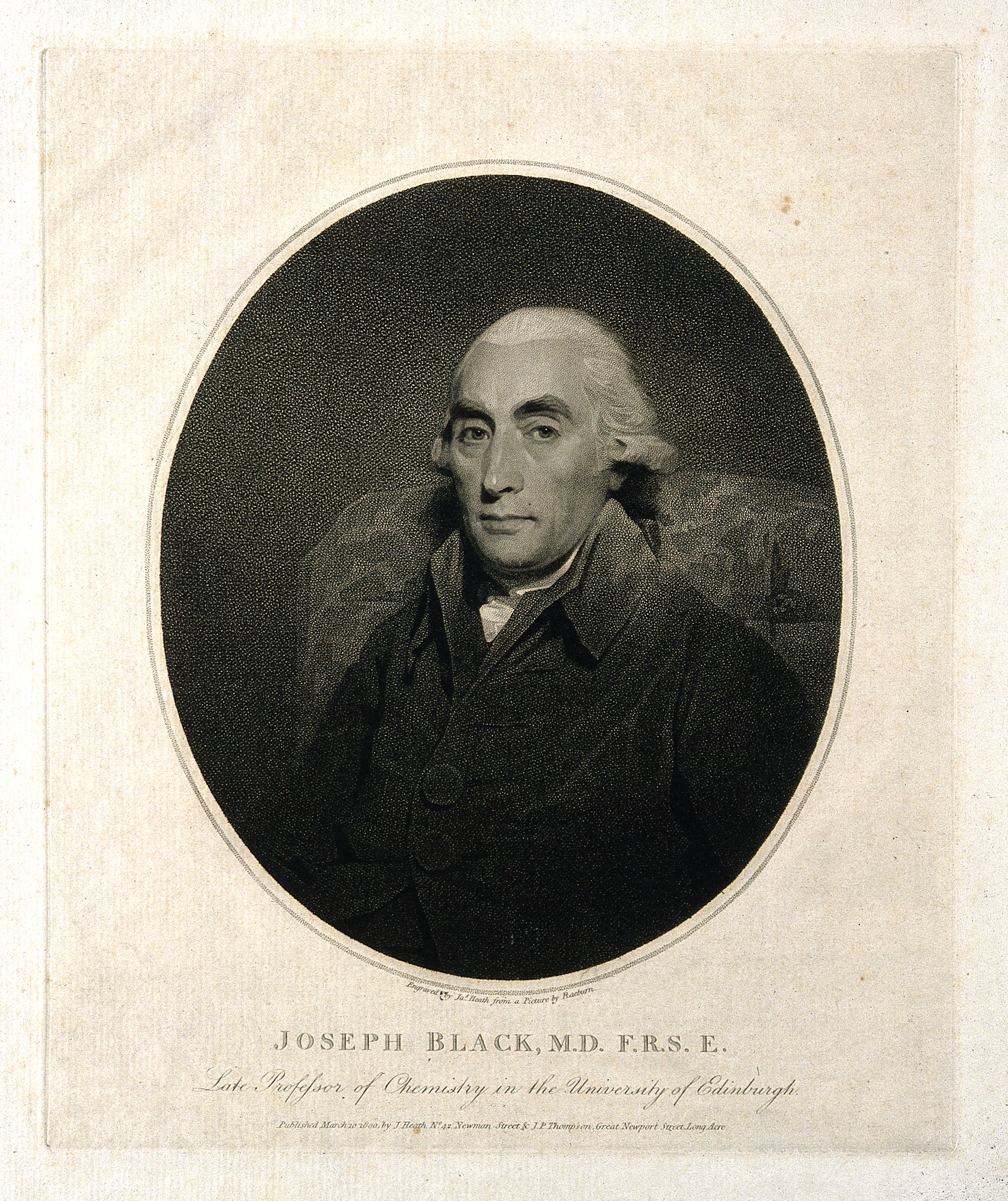
Figure: Joseph Black (1728–1799). Black was a physician and chemist at Glasgow, then Edinburgh. Stipple engraving by James Heath after Henry Raeburn, 1800 (Wellcome Collection / Wikimedia Commons, public domain).
Black lectured in medicine and chemistry, in the mid eighteenth century he was based in Glasgow, where he was a contemporary of James Watt. His work on heat was done while he was still a physician. It was published posthumously by John Robison as Lectures on the Elements of Chemistry (Edinburgh, 1803) (Black, 1803).
Thermometers had existed since about the 17th century. This leads to a mystery: ice melts, but the temperature doesn’t change. The same thing happens at the other end: water boils, steam is produced, and the thermometer sits at the boiling point. If you heat an equal mass of water equally as a mass of mercury, they do not change temperature equally. The important step that Joseph Black made was to realise that temperature and heat are separate quantities. That is quite a big leap. Most children, and most of us at first, think heat and temperature are the same. Temperature is a reading, but heat is a quantity that can enter a body without changing the reading.
Black’s notion is that heat is a quantity you can add, mix, and hide. Take known masses, mix them, and they come up to a final temperature: the heat has mixed. Capacity is when something absorbs heat at a different rate. Mercury, he says, has less capacity for the matter of heat than water: the same heat produces a larger change of temperature. That is specific heat. The ice can start below zero, but once you get it to zero it stops absorbing heat — it is swallowing heat, latent heat. The heat that turns water into steam does not raise the thermometer either. Recovered when the change of state is reversed.
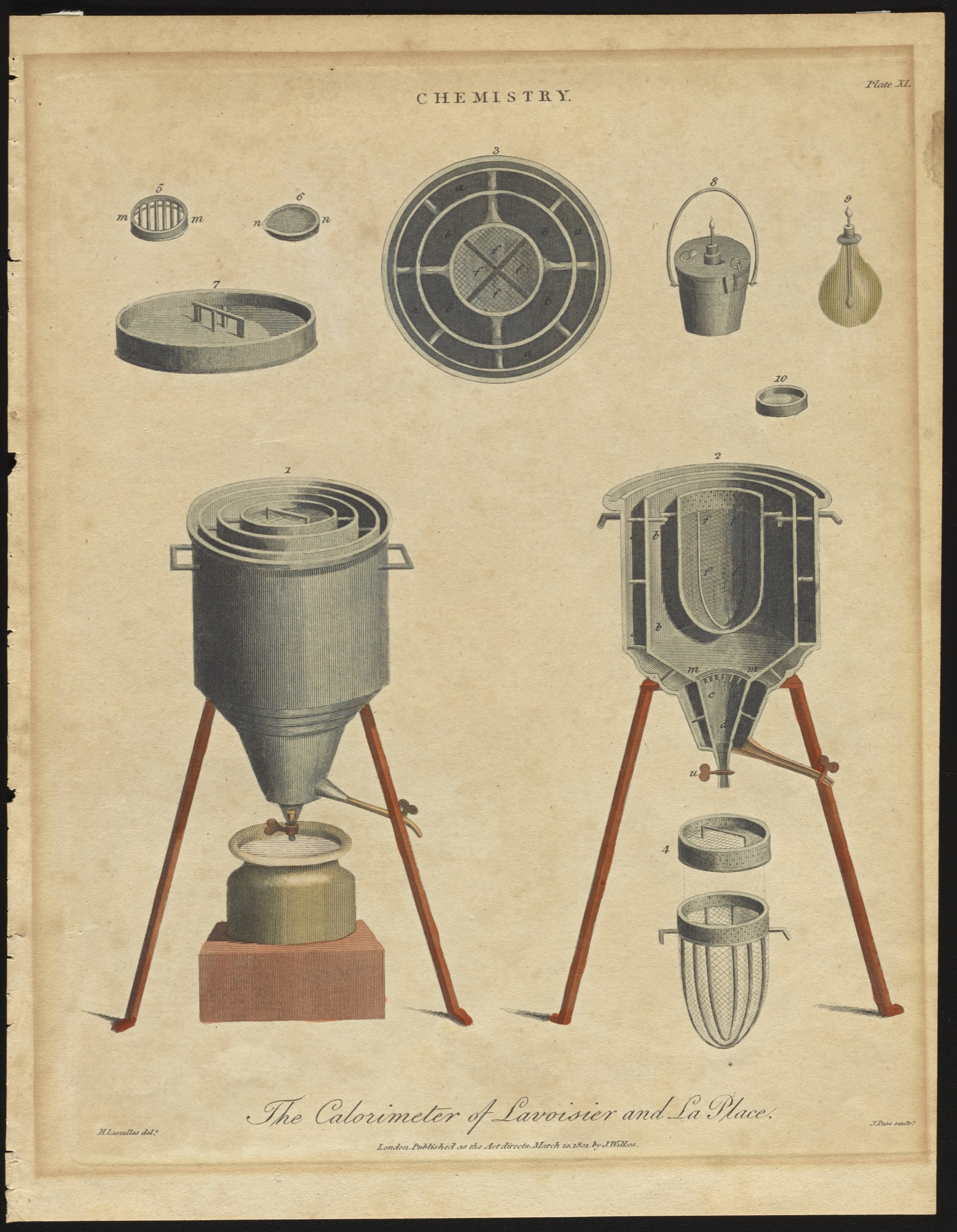
Figure: The calorimeter of Lavoisier and Laplace. Heat delivered is read as the mass of ice melted; the conversion factor is Black’s latent heat of fusion. Plate XI from Encyclopaedia Londinensis (1801–02), after H. Lascelles (Wikimedia Commons / Science History Institute, public domain).
Black did not build this box. His own apparatus was an open fire and a pan. He tried to keep the fire steady — bellows, not a closed system — and timed how long it takes to melt ice or to boil a pan dry. The ice calorimeter is Lavoisier and Laplace in the winter of 1782–83: a sample in the inner chamber, a jacket of ice, an outer ice shield against the room. Heat that leaves the sample melts ice in the middle jacket; you weigh the meltwater. The conversion factor is Black’s latent heat of fusion: the heat that would raise an equal mass of water by about \(143\)–\(144\) Fahrenheit degrees. That is a quantity of heat, not a temperature on the thermometer. It is close to the modern figure of \(80^\circ\mathrm{C}\), or \(334\,\mathrm{kJ\,kg}^{-1}\). The thermometer is no longer the meter. The meltwater is.
One of the striking things in this period, even though Britain and France are at war half the time, is how much scientific traffic there is between them, including people travelling. Laplace is famous in England. Lavoisier, with Laplace, forms an early table of chemical elements; Lavoisier is killed in the Revolution; Laplace survives it and later becomes a count under the Bourbon restoration. Their calorimeter is inspired by Black.
Black’s unit of heat is not a temperature. It is the heat that raises an equal mass of water by one degree on Fahrenheit’s thermometer. On that scale the interval from melting ice to boiling water is \(180\) units. The extra heat to turn the boiling water into steam he estimates at about \(810\) of those units: the pan sits on the fire four and a half times longer boiling dry than it did coming up to the boil — say fifteen minutes to the boil, then about an hour and a quarter to evaporate. He knows the timing method is rough because the fire is not a closed system. His contemporary, James Watt, condensing steam and measuring the water it warms, gets nearer \(950\), within a few percent of the modern figure. The modern figure is about \(967^\circ\mathrm{F}\) on the same scale, \(540\,\mathrm{cal\,g}^{-1}\), or \(2256\,\mathrm{kJ\,kg}^{-1}\): a little more than five times the heat that takes water from \(0\) to \(100^\circ\mathrm{C}\).
The number is already important industrially. Until Watt, a Newcomen engine condensed steam by spraying cold water onto the cylinder. That makes a vacuum and the piston comes down; then you heat the cylinder again and it goes up. The condensation on the cylinder is latent heat the engine has to repay on every stroke. Watt’s question is: how much energy is that spray? His answer is the separate condenser — take the steam out of the cylinder and cool it somewhere that is always cold. That is why the engine becomes more efficient. Manufacturing it takes him twenty-five to thirty years. Glasgow does not yet have the machinery; he has to come to Boulton in Birmingham. You do not see these engines in industrial use until about twenty years after the 1760s work. The Lap engine in the Science Museum in London is late 1770s, early 1780s.
Sadi Carnot and the Fall of Heat
Black made heat a quantity you can add, mix and hide. From our perspective, the next step comes from Sadi Carnot (1796–1832). Carnot has a practical question, he’s not focussed on what heat is made of, he wants to understand the limits of a steam engine.
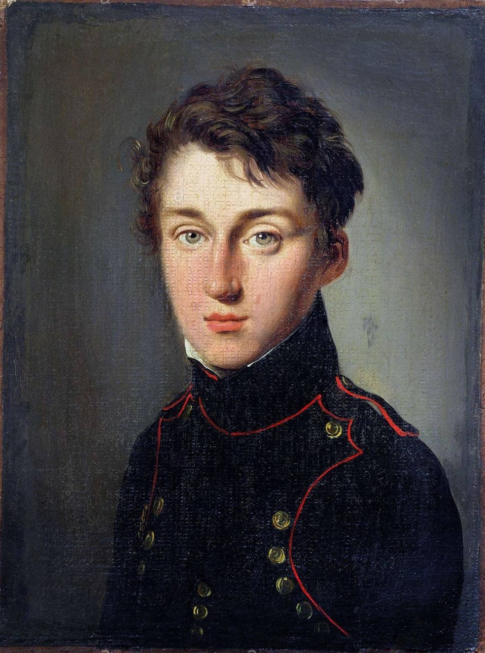
Figure: Sadi Carnot (1796–1832), aged 17, in the uniform of the École Polytechnique. Portrait by Louis-Léopold Boilly, 1813 (Wikimedia Commons, public domain).
Nicolas Léonard Sadi Carnot was a military engineer, son of Lazare Carnot. Lazare who was a mathematician and the “Organizer of Victory” of the Revolutionary armies. After Waterloo Lazare he was driven into exile, and Sadi’s career in army under the Bourbon restoration stalled. The portrait is a decade before the book. By 1824 he is on reduced pay in Paris, attending lectures at the Conservatoire, and paying himself to print six hundred copies of a short essay: Réflexions sur la puissance motrice du feu (Carnot, 1824).
After his time in Glasgow, James Watt had moved to Birmingham and together with Matthew Boulton, commercialised a more efficient steam engine. By the 1820s the steam engine was widely used in mines, mills, looms and forges. Carnot believes that one day it will serve as a universal motor, but he notes that it doesn’t have a theory of mechanics. France is watching Britain do steam better. Watt’s engines are a few percent. One reason they stay that low is that he refused high-pressure steam: he thought it was dangerous, and his patent covered engines that were not high-pressure. He was probably right about the boilers they could manufacture then. Later, corrugated boilers, high temperature and high pressure, and a modern steam turbine is about sixty percent. The so-called “practical men” are improving the machine, but Carnot wants to know whether any of that can be unbounded, or whether there is a ceiling independent of the machine and of the substance that runs through it. That is the same kind of question we would like to be able to ask of intelligence. We are in almost the same position he was in: a load of our quantities are not defined.
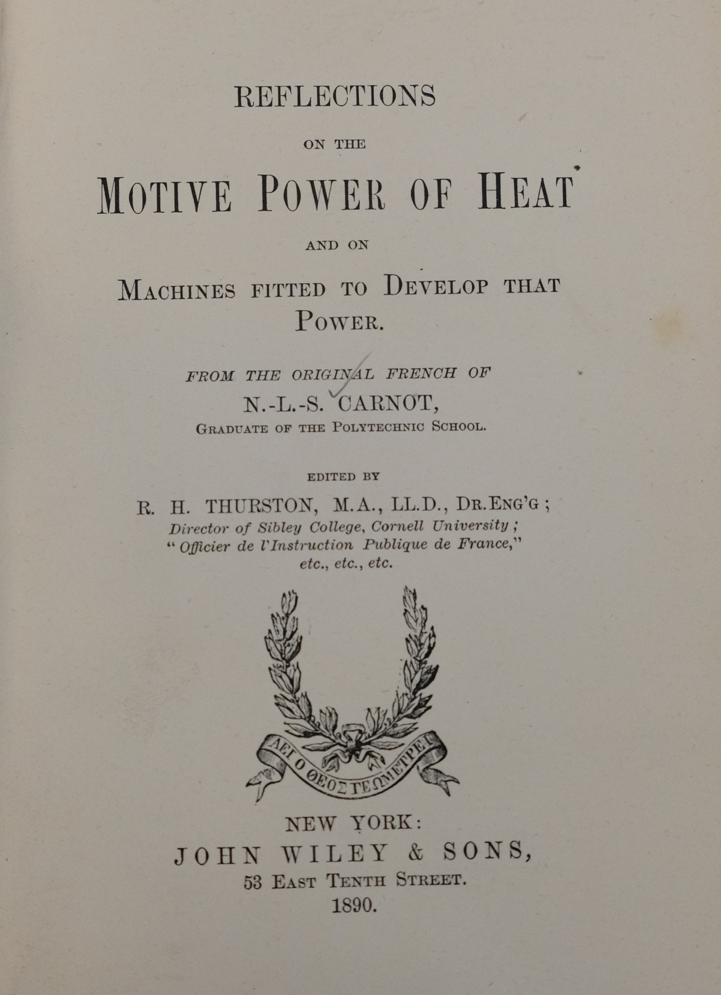
Figure: Title page of R.~H. Thurston’s 1890 English translation of Carnot’s 1824 Réflexions sur la puissance motrice du feu. The original was printed in Paris by Bachelier, at Carnot’s expense, in six hundred copies.
The 1824 original is a short book, 118 pages, almost unread in his lifetime. Thurston’s translation is how most English readers met it. The argument does not depend on calculus. It depends on a picture of heat that Black had made plausible: caloric, a conserved fluid, falling from hot to cold.
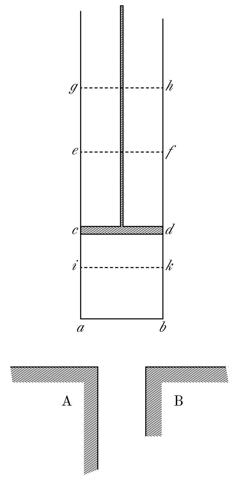
Figure: Carnot’s own figure of the mill (1824). The cylinder \(ab\) holds the working body; \(cd\) is the piston. Body \(A\) is the furnace, body \(B\) the refrigerator — two reservoirs of caloric at different temperatures. Caloric taken from \(A\) is given up to \(B\). Vectorised from the plate in Réflexions sur la puissance motrice du feu (Wikimedia Commons, public domain).
Carnot’s own comparison: the motive power of heat can be compared to that of a waterfall. A waterfall has a maximum you cannot exceed, whatever machine you put in the stream. The power depends on the quantity of water and the height of the fall. Heat, likewise, depends on the quantity of caloric and on what he calls the height of its fall — the difference of temperature between the bodies exchanging it. In English, mill until relatively recently also meant a factory; the picture here is a water mill. In a steam engine the boiler is the upper reservoir, the condenser the lower. Carnot’s own plate is that mill: body \(A\) the furnace, body \(B\) the refrigerator, the cylinder the wheel. The caloric developed in the firebox is taken up by the steam, passes through the cylinder, and is given up to the cold water. The mill turns because the caloric moves. The same quantity that left the hot reservoir arrives at the cold one: heat moving like water does in a waterfall. Conceptually he is thinking of the fall of water driving a wheel, rather than a direct conversion of some of the heat into the work. He is honest that he does not fully understand how the work comes from the fall of caloric. Watt already knows, from Black, that steam carries latent heat around and gives it up when it condenses. What is surprising, looking back, is that this conservation theory of heat exists before conservation of energy.
He pays for six hundred copies. In the summer of 1832 he falls ill; he dies of cholera on 24 August, at Ivry, aged 36. The book, and the work, almost vanish with him. Two years later Émile Clapeyron, another polytechnicien, recasts the argument in 1834 in the language of indicator diagrams, and people form what becomes known as the caloric theory of heat — the dominant theory, a conservation theory before conservation of energy.
Count Rumford’s Cannon
Carnot treated heat as a conserved fluid because that is what a mill requires. The difficulty with that picture was already in print. In 1798, twenty-six years before the Réflexions, Benjamin Thompson, who styled himself Count Rumford, published a paper in the Philosophical Transactions on heat excited by friction (Rumford-friction98?).
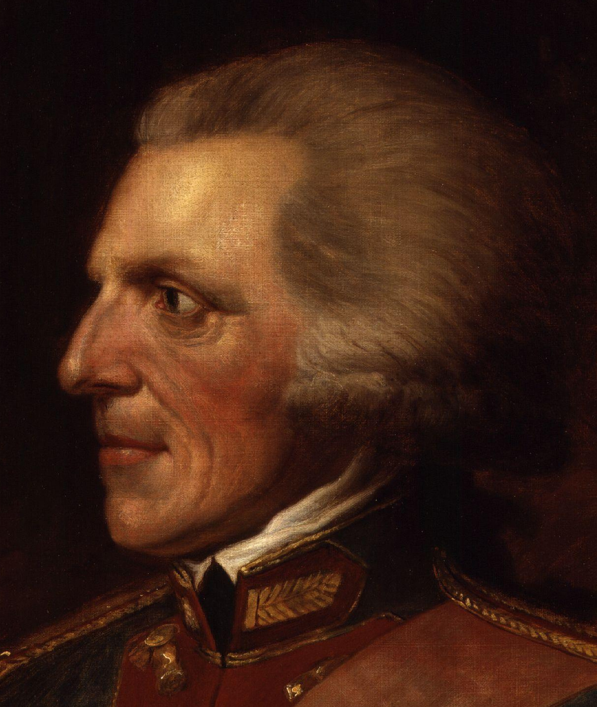
Figure: Benjamin Thompson, Count Rumford (1753–1814). American-born, then in the service of the Elector of Bavaria. Portrait by Moritz Kellerhoven (Wikimedia Commons, public domain).
Rumford was born in the United States and becomes superintendent for the boring of brass cannons in the military arsenal at Munich, in the service of Bavaria. An American working for a German army, submitting to the Royal Society. He is struck by how hot the gun becomes, and by how much hotter the metallic chips are (he checks and they are hotter than boiling water). If heat were conserved, perhaps the shavings have lost caloric and the cannon has gained it. He measures the specific heat of the shavings and of the cannon and finds they are the same. His paper to the Royal Society asks where the heat is coming from.
He asks whether the chips have changed their capacity for heat, as Black’s latent-heat doctrine would require if caloric were being squeezed out of the metal, but he finds they haven’t. He builds an experiment with a short hollow cylinder is turned against a blunt steel borer by machinery carried round by horses. A wooden box filled with water surrounds the cylinder. At one hour the water is at \(107^\circ\mathrm{F}\); at two hours \(178^\circ\mathrm{F}\); at two hours thirty minutes it boils.
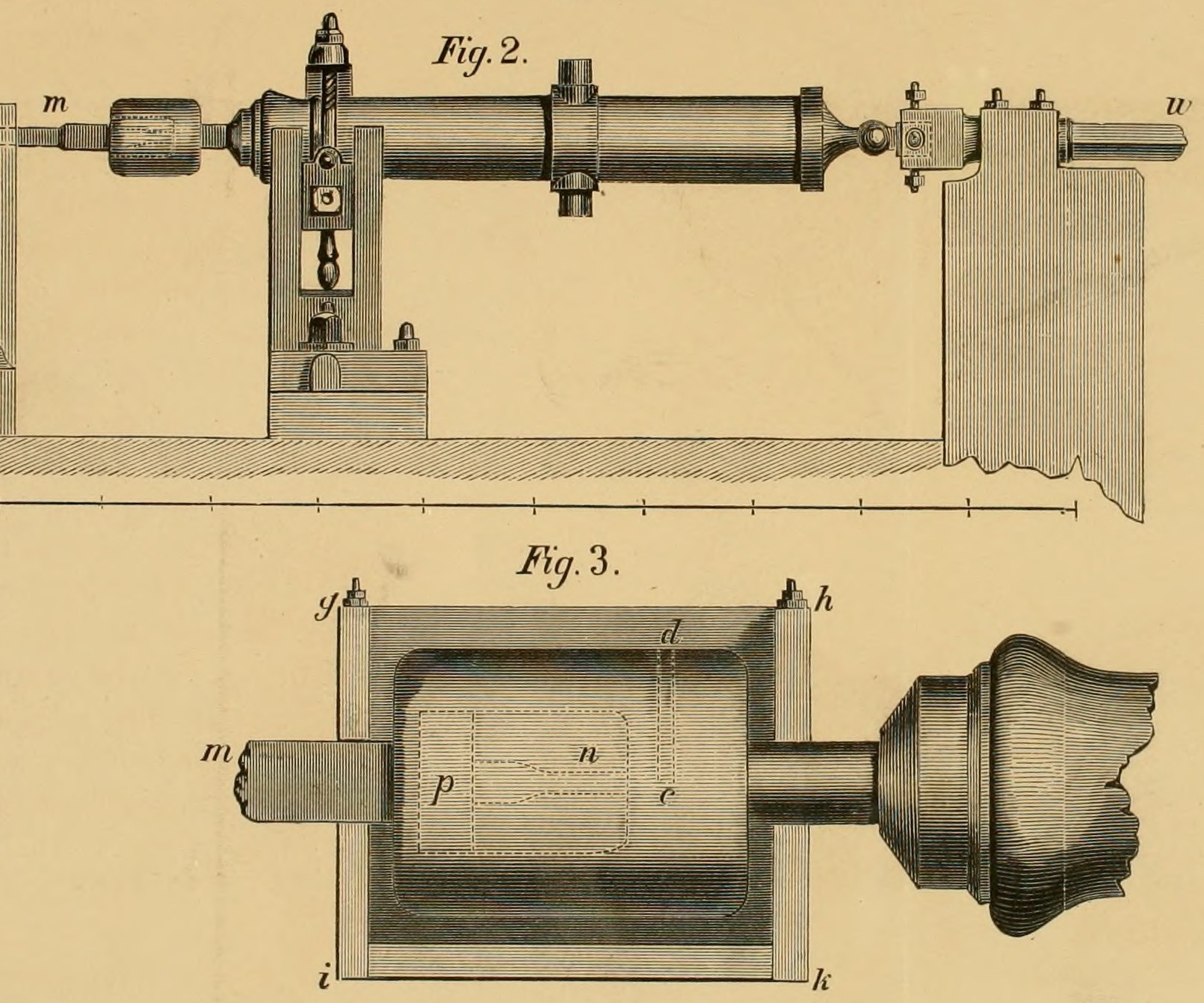
Figure: Rumford’s 1798 apparatus, as reprinted in The Complete Works of Count Rumford (1870). Fig.~2: the cannon in the boring machine, turned by the bar \(w\). Fig.~3: the same cylinder in the water box that is brought to the boil.
Rumford remarks that the source of the heat generated by friction appeared evidently to be inexhaustible. But anything which an insulated body can continue to furnish without limitation cannot possibly be a material substance. That is 1798. Caloric is in the table of the elements. Lavoisier, with Laplace, is the person who names oxygen, previously phlogiston; he was a smart person, and caloric still sat in the table. Rumford’s conclusion is that heat is a mode of motion — a kinetic theory of heat. For what we are looking at here, that is the form of heat: the air in this room is hot because it is in motion. Heat at some point also becomes radiation; ignore radiation for the moment. It is a qualitative blow to caloric, not a mechanical equivalent. He does not weigh a known quantity of work against a known quantity of heat. He does not say where the heat is coming from. He sets it up as an example against the theories of conserved heat.
Mercury, Ice, Steam, and Air
Black already treats temperature as a reading and heat as a quantity. The reading, in the 1840s, comes from one of three expansion thermometers. Fahrenheit and Celsius use mercury. Accurate laboratory work uses air. All three pin two fixed points — ice and steam, or a close cousin — and then divide the interval so that equal expansions of the chosen substance are equal degrees. Thomson will inherit that practice, and then refuse it as a definition of a degree.
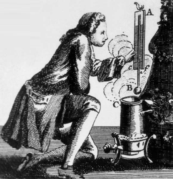
Figure: Daniel Gabriel Fahrenheit (1686–1736) with a mercury thermometer. Anonymous engraving, 18th century (Wikimedia Commons, public domain). The instrument is mercury in glass; the scale is equal expansion of that mercury between two pins.
Fahrenheit’s mercury thermometer is the household instrument of the eighteenth century. He marks a mixture of ice, water and sal-ammoniac as \(0\), and (originally) blood heat as \(96\). The scale that survives is a recalibration of the same tube: ice at \(32\), steam at \(212\), so there are \(180\) equal expansions of mercury between the two pins. Celsius, in 1742, uses the same pins on a centesimal division. His own numbering ran the other way — \(100\) at ice, \(0\) at steam — and was inverted within a few years. By Thomson’s time ``Celsius’’ means ice \(0\), steam \(100\). The physics is the same as Fahrenheit: you have chosen a substance, and you have called equal expansions of it equal degrees. Black’s whole point is that this reading is not the quantity of heat. The same rise of the same mercury takes different heat in water, in oil, in ice that is melting.
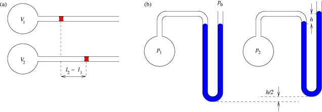
Figure: (a) Constant pressure: a sliding mercury index, open to the room; the volume of the trapped air is the reading. (b) Constant volume: a mercury manometer; the height \(h\) is the reading. Scheme by P. Peterlin (Wikimedia Commons, CC BY-SA 3.0). Thomson’s 1848 comparison is with (a).
The air thermometer is the 1840s laboratory standard, the scale to which mercury and alcohol are reduced (Regnault). Take a glass bulb of dry air and confine it with mercury. The mercury is open to the room: either a sliding thread in a capillary, as in (a), or a cistern you raise and lower. You move the mercury until the two surfaces sit at the same height, so the trapped air is at atmospheric pressure. The volume of that air is then the reading. Ice water and steam still fix two points; the interval is divided so that equal increases of volume are equal degrees. That is Gay-Lussac made into an instrument: far from condensation, the volume of air rises almost linearly with this temperature. Push the same line far enough and the volume would vanish at about \(-273^\circ\) of the air scale. That number lives in the instrument, not in Carnot. Panel (b) is the other common form, a constant-volume gas thermometer, where you read pressure from the manometer height. Thomson in 1848 is arguing with (a). Air is a better expansion-substance than mercury — different gases agree closely unless they are about to liquefy — but it is still a substance. A degree that means ``equal expansion of air’’ is not yet independent of the thermometer.
Thomson’s Scale from the Mill
William Thomson, who later became Lord Kelvin, takes Carnot seriously as theory. In 1848 he is a twenty-four year old professor of natural philosophy at Glasgow, and he has read Clapeyron’s recasting of the Réflexions. Fahrenheit, Celsius and the air thermometer already exist: ice and steam already mark \(0\) and \(100\) on the scale he will compare against. Those pins are a century old. What does not exist is a meaning of degree that is independent of mercury, or of air. If the motive power of heat depends only on the quantity of caloric and the height of its fall, then that height should be usable as a thermometer (Thomson-absolute48?). That is what he adds at twenty-four: a definition of the interval, not a new pair of fixed points, and not a bottom of the fall. The 1848 answer still assumes that heat is conserved. It is not yet the scale that later bears his name.
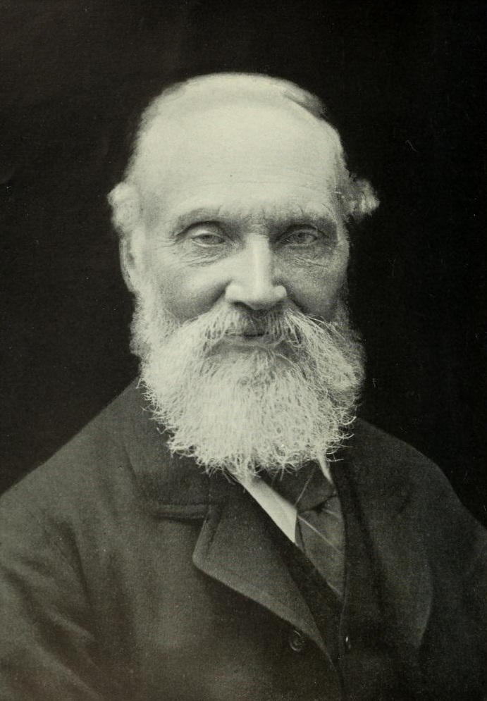
Figure: William Thomson (1824–1907), later Lord Kelvin. Photograph from The World’s Work, 1902 (Wikimedia Commons, public domain) — half a century after the 1848 scale.
Thomson studied as an undergraduate at Cambridge and spent his career as professor of natural philosophy at Glasgow. Maxwell is a younger contemporary in the same group: people who combined the empirical work going on in places like Glasgow, where they really cared about the engineering, with a deep mathematical understanding. In 1848 Thomson is looking for a thermometric scale that is not an accident of mercury or air. He believes that Carnot’s theory provides such a scale. He already has a quantity of heat: Black’s unit, the heat that raises a kilogramme of water by one degree of the air thermometer. What he still lacks is a meaning for an interval of temperature that does not belong to one substance. When he is twenty-four he tries to interpret the degree as a measurement related to specific heat: how much work could you extract from one unit of Black’s heat falling one degree. Carnot’s mill supplies it: the motive power of a given quantity of caloric falling through one degree. That is mill-work from a fall, as water on a wheel.
The air thermometer is the scale Thomson is arguing with. Household thermometers use mercury because it is convenient; in accurate work you compare the mercury against air and quote the air reading (Regnault). Air is a better expansion-substance than mercury, but it is still a substance. A degree that means ``equal expansion of air’’ is not independent of the thermometer. Thomson will not call that absolute.
What he adds is a meaning for the interval. Take a unit of heat — Black already told you how to measure that — and let it fall through Carnot’s mill. Call one degree whatever drop of temperature always yields the same motive power from that unit, whether you are near steam or near ice. The degree now belongs to the mill, not to mercury, and not to air. Independence of substance here means independence of the thermometer’s fluid and of the engine’s working fluid. The fixed points stay where Fahrenheit and Celsius left them. That is why the paper matters in 1848, before anyone has broken conservation of heat.
Thomson’s own statement of the characteristic property: all degrees have the same value; a unit of heat descending from a body \(A\) at temperature \(T^\circ\) to a body \(B\) at \((T-1)^\circ\) gives out the same mechanical effect, whatever the number \(T\). That is the mill, turned into a ruler. The working fluid is still caloric. The fall is still a fall, not a conversion. He then compares the new ruler with the air thermometer, using Clapeyron’s formulae and Regnault’s steam data. The two scales are forced to agree at ice and at steam. Everything else is a table of how unequal an air-thermometer degree is, in mill-value, as you go up the scale. Work is how we make the degrees equal. It is not how we make the heat, and it is not a new zero.
The \(-273^\circ\) that looks like absolute zero is already sitting in the air thermometer — the same bulb of air, volume as the reading. If that volume is linear in temperature, pushing the graduation far enough reduces the air to nothing at \(-100/0.366\), which Thomson writes as \(-273^\circ\). He uses that fact only as a reason why Clapeyron’s table was to be expected: an air-thermometer degree is worth more when it is cold, because a finite number of those degrees is trying to reach infinite cold. It is not the zero of his scale, and he does not compute a table down to it. On the mill scale a unit of heat can always be let down one more equal-value degree, and still arrive. Infinite cold is at \(-\infty\). 1848 has done something narrower: it has made a degree a Carnot object. There is not yet a bottom, because caloric is still conserved.
Thomson writes that in the present state of science no operation is known by which heat can be absorbed without either raising a temperature or becoming latent. Conversion of heat, or caloric, into mechanical effect is probably impossible, certainly undiscovered. Actual engines must therefore look for their power not in absorption and conversion, but in the transmission of heat. That is Carnot, stated as a fact of 1848, and it is the assumption his mill-degree rests on.
Joule and the Mechanical Equivalent
James Prescott Joule (1818–1889) gives the answer to Rumford’s riddle. He theorises that a measured quantity of mechanical work could create a measured quantity of heat. If it can then heat is not a conserved fluid. This would imply that Carnot’s mill becomes a special case, not the general law. Joule is a Manchester brewer who tries this experiment with a paddle wheel (Joule-equivalent50?).
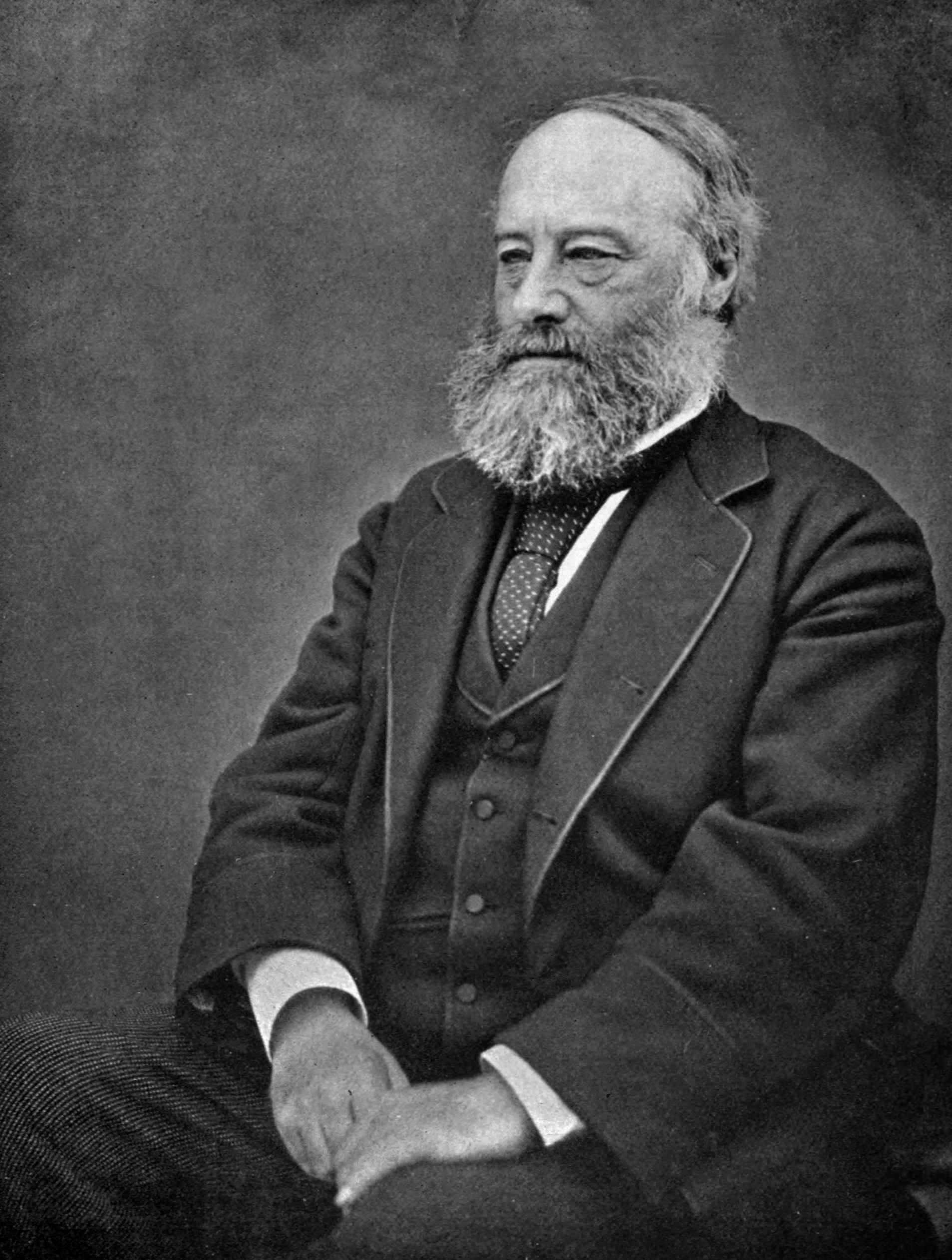
Figure: James Prescott Joule (1818–1889). Seated portrait, later in life (Wikimedia Commons, public domain).
The family brewery is in Manchester where Joule has a private laboratory. From 1840 he is working to relate heat to electricity and to chemical affinity. In 1843 he argues that the heat from magneto-electricity is proportional to the work absorbed. Mayer, in 1842, has already claimed that agitating water warms it, without a measured force. Joule wants the equivalent.
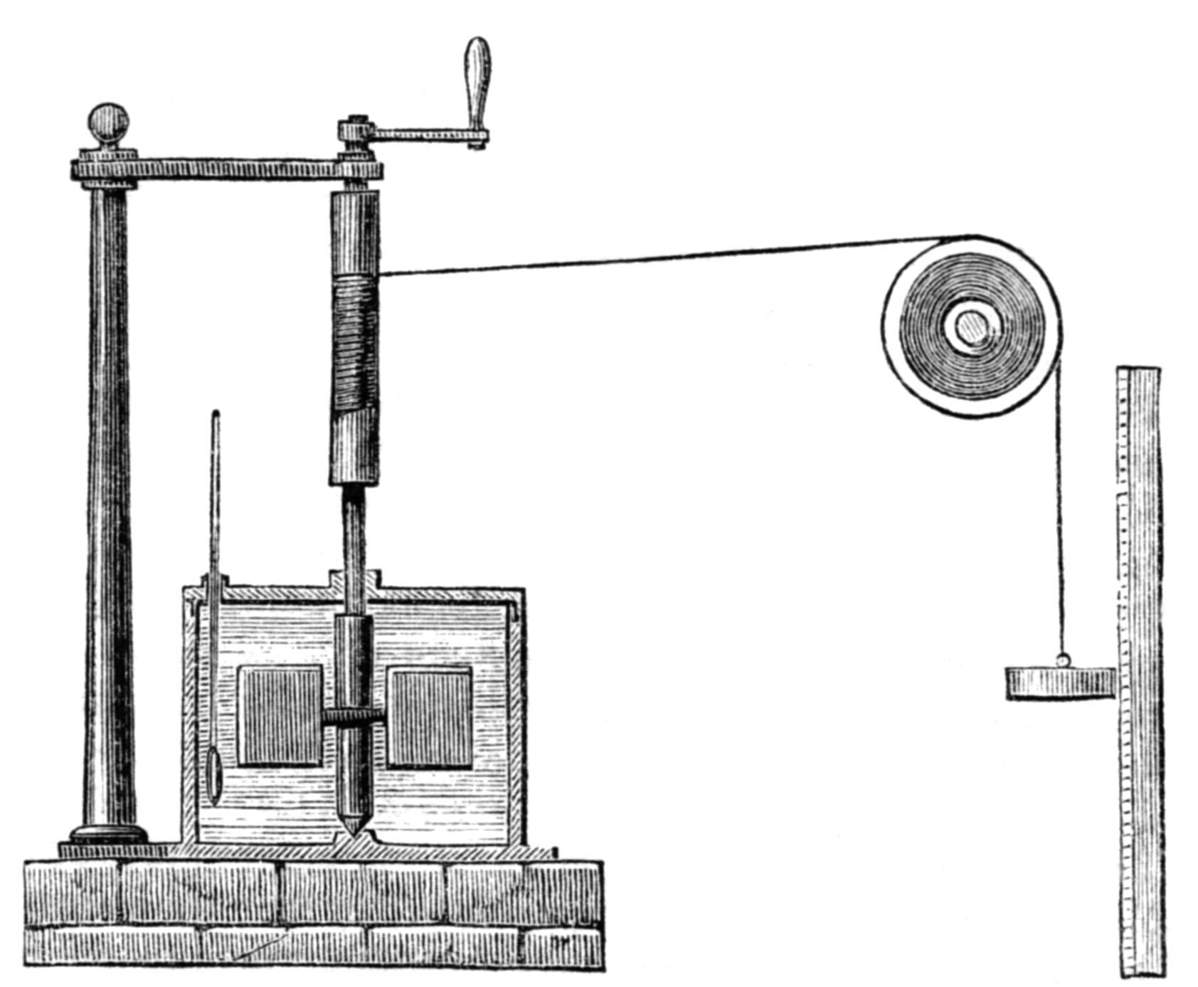
Figure: Joule’s apparatus for the mechanical equivalent of heat. A falling weight turns a paddle in water; the work is known, the rise in temperature is measured. Engraving from Harper’s New Monthly Magazine, August 1869 (Wikimedia Commons, public domain).
In Joule’s apparatus weights descend and turn a paddle in a can of water. The work associated with dropping a mass through a height is \(mgh\). It is coiled around a bearing; there is a water paddle in a tank. To do the experiment you try to get rid of friction in the spindle. He did not drop it once: he had to drop it multiple times to show how much work converted into heat. It is a very similar experiment to Rumford’s, but he has a better thermometer (mercury or other liquid, not air, by the look of the apparatus) and he is measuring the specific heat capacity of water. Mechanical power is being spent, and heat appears. Finally people realise that heat energy and work can transform into one another. That is the 1840s. Not very long ago.
Cambridge here is the British Association meeting of June 1845, not the Cambridge Philosophical Society — that society is Thomson’s 1848 scale. Joule exhibits the brass paddle to the Chemical Section; the published letter opens by saying so (Joule-equivalent45?). That run gives about \(890\) foot-pounds per degree per pound of water. He also uses other methods such as magneto-electricity, rarefaction of air, passing water through narrow tubes to give neighbouring figures. His mean estimate is near \(817\). By 1850 the number is settled as \(772.692\) foot-pounds (Joule-equivalent50?). The scientific world, he notes, preoccupied with the hypothesis that heat is a substance, had almost unanimously denied that fluid friction could generate heat.
You will hear people say that when they built steam engines they had no theory of thermodynamics. That is not true. They had theories of thermodynamics. They did not have complete theories. We may not have a complete theory of thermodynamics today. This is where we are with machine learning: we do not have good theories of what is going on in the models, and we do not even have good definitions of intelligence. People can go around saying AGI or superintelligence, and it does not mean very much. Caloric is better defined. At least caloric is a notion you can look at and say: it is not conserved. It is telling you something specific you should expect. It is falsifiable. If you do not define your terms, you cannot do falsifiability.
Once you realise that Joule converts work to heat, you also get the sense that heat converts to work. You can convert all your work into heat. You cannot get all the heat back as work. Carnot is assuming that the work comes from the fall, as in a mill. Here the heat itself converts. You cannot keep that theory of heat engines and Joule’s demonstration as general laws. Clausius in 1850, and Thomson in 1851, will keep Carnot’s limit and drop conservation of heat. We take Clausius first: two laws, and \(\mathrm{d}Q/T\). Thomson then returns: the 1851 dynamical theory first, and with Joule in 1854 a scale that has a bottom.
Clausius and \(\mathrm{d}Q/T\)
Heat is not conserved. Carnot’s limit remains. That is the problem Clausius inherits from Joule and Thomson. If the caloric mill is gone, what still closes when a reversible engine runs a cycle? The answer is not a quantity of heat. It is heat divided by temperature. A reversible cycle produces no entropy.
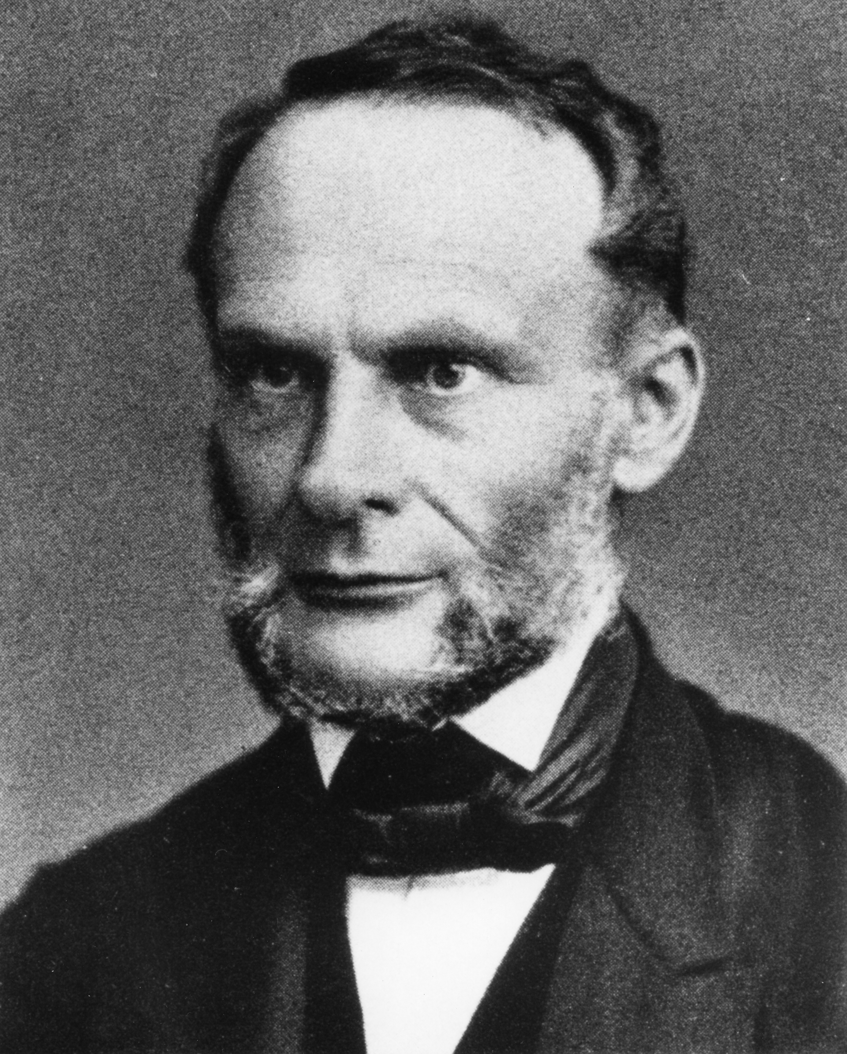
Figure: Rudolf Clausius (1822–1888). Photograph from the AIP Emilio Segrè Visual Archives, Lande Collection (Wikimedia Commons, CC0).
Clausius is a mathematical physicist, first in Berlin, later Zurich, Würzburg and Bonn. It is quite close between Kelvin and Clausius to get to the formula. In 1850, independently of Thomson’s 1851 dynamical theory, he writes the two laws (Clausius-motive50?). He holds on to Joule’s equivalent between work and energy, keeps Carnot’s limit, and drops the notion that heat is conserved. He is doing all this without a notion of conservation of energy, which is gobsmacking. Bernoulli too: \(PV=NRT\) is later; he was doing it with momentum. The first law is Joule’s equivalent made universal: heat is a form of work. The second is what remains of the mill: heat does not pass from cold to hot by itself, and no cyclic engine converts the heat of a single bath entirely into work.
The first law is why \(\oint \mathrm{d}Q\) is not zero for an engine. Some of the heat taken from the hot bath does not arrive at the cold bath; it has become work. That is Joule, inside Carnot’s cycle. The second law is why you still cannot take all of it. There is a remainder that must be rejected to the cold bath, and the size of that remainder, for a reversible engine, depends only on the two temperatures — not on whether the working substance is steam, air, or anything else. That was Carnot’s other claim, and it survives.
Thomson and Joule’s 1854 scale is this statement: the absolute temperatures stand in the same ratio as the two heats. What Clausius notices is that in a reversible engine the heat energy at the hot temperature, divided by that temperature, equals the heat energy at the cold temperature, divided by that temperature, as you go around. If the cycle is reversible, that quantity is conserved: the integral of the small changes in heat, over the whole loop, is zero. That is what Clausius told us. If the cycle is irreversible, the same integral, with \(\mathrm{d}Q\) the heat absorbed by the working substance, is strictly negative. It is never positive on that convention. Clausius’s 1854 paper calls the quantity the equivalence-value of the transformation (Clausius-equivalence54?); his uncompensated transformation is the negative of the integral, and is \(\ge 0\).
If every reversible cycle gives zero, the integral of \(\mathrm{d}Q/T\) between two states cannot depend on the reversible path you take. That is the definition of a state function. Clausius writes \[ S - S_0 = \int \frac{\mathrm{d}Q_{\mathrm{rev}}}{T}. \] Heat \(\mathrm{d}Q\) is not a state function: the heat you put in depends on the path, which is why \(\oint \mathrm{d}Q\) is the work of the engine. Dividing by \(T\) along a reversible path removes that path-dependence. Reversibility is the condition. It means the engine can be run backwards and the baths restored: no finite drops of temperature, no friction, no paddle wheel hidden in the mechanism.
This is the mill, rewritten after Joule. The working fluid comes home. Its entropy comes home with it. The hot bath has lost \(Q_h/T_h\); the cold bath has gained \(Q_c/T_c\); those two are equal. No transformation has been left over. Reversible does not mean ``nothing happened.’’ Work was done. It means the transformation can be undone, and when you close the loop there is no residue.
An irreversible cycle is still a cycle: the working substance returns, so its \(S\) is unchanged. What has changed is the baths. You took \(Q_h\) from the hot bath and, because some of the fall was wasted, you delivered more than the reversible \(Q_c\) to the cold bath. The integral \(\oint \mathrm{d}Q/T\), with \(\mathrm{d}Q\) the heat absorbed by the working substance, is then strictly negative (Clausius-equivalence54?). Equivalently, the entropy lost by the hot bath is less than the entropy gained by the cold bath. The difference was produced. Clausius’s uncompensated transformation is the negative of this integral: it is \(\ge 0\), and it is strictly positive when the cycle is irreversible.
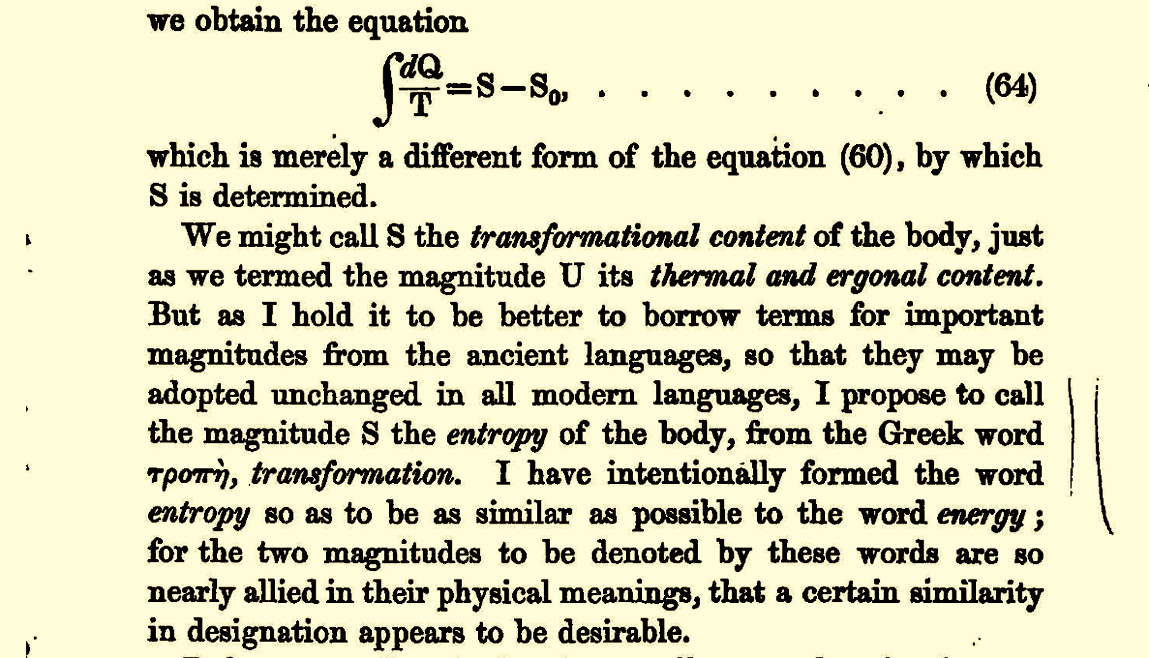
Figure: Clausius names entropy, 1865. English translation of the memoir: \(\int \mathrm{d}Q/T = S-S_0\), from Greek τροπή, transformation. He forms the word to sit beside energy.
In 1865 he gives the state function a name (Clausius-entropy65?). Clausius writes that we might call \(S\) the transformational content of the body, just as we term the magnitude \(U\) its thermal and ergonal content, the inner energy; but that it is better to borrow terms for important magnitudes from the ancient languages, so that they may be adopted unchanged in all modern languages. He proposes to call \(S\) the entropy of the body, from the Greek word τροπή, transformation. He has put an \(n\) on the front. He says explicitly that he has formed the word to be as similar as possible to energy, because the two magnitudes are so nearly allied in their physical meanings that a certain similarity of designation appears desirable. They are not allied because of the division by \(T\). There is no Boltzmann’s constant here yet: this is a macroscopic property, something he can derive from measuring what was lost, or noticing it is not lost in a reversible cycle. He has no notion underneath it that this is anything to do with uncertainty. He just says: I need this piece to fit the puzzle. The assumption, coming at it afterwards, is that they were looking at energy conserved and therefore this piece is missing. It is not quite like that.
Clausius did not give the Boltzmann distribution, and he did not make entropy a measure of uncertainty. He gave the macroscopic balance that any later prescription must respect. \(S\) is a macroscopic measurement that is extensive: the entropy of a system increases as we increase the size of the system. Temperature is intensive: it does not. When we write \(p_i \propto e^{-\beta E_i}/Z\) and later derive it from MaxEnt, read it as a statistical answer to a constraint he already framed: fixed mean energy, maximum entropy, no perpetual motion. The historical chain is engines, then the equivalent, then this integral, then statistics, then information.
Later, Maxwell, then Boltzmann and Gibbs, come to the same sort of conclusions. This century, Shannon and Jaynes reuse the functional form for what might be said to be a different job. Shannon is always discrete. Wiener is continuous. Wiener never drops the mechanism behind the entropy: he always thinks about what drives the distribution. In Shannon you just say it is a probability. A lot of the theory does not have to specify what the probability is; you use that it normalises to one and is positive, and you derive a lot from that. That is mathematics. The other bit, where you have to talk about mechanism, is physics.
Thomson Returns: The Scale After Joule
Clausius has kept Carnot’s limit and dropped conserved heat. Thomson does the same, independently, a year later. In 1851 he writes the dynamical theory of heat (Thomson-dynamical51?). The mill is still there. The 1848 ruler is not: that scale assumed a conserved unit of heat, and Joule has broken the unit. What replaces it is a ratio of the two temperatures to the two heats. Thomson and Joule write that second scale in 1854, and for the first time the fall has a bottom.
The 1848 paper had already heard of Joule, in a footnote, and had refused him: conversion of heat into work was probably impossible, certainly undiscovered. The paddle wheel is the experiment Thomson said had not been shown. By 1851 he accepts it. Heat can be generated by work, and some of the heat taken from the hot bath does not arrive at the cold bath — it has become work. Conservation of caloric cannot be the general law. Clausius had already said so. The 1851 paper is that acceptance, and Thomson’s form of the second law. The rewrite of the scale waits until 1854.
In 1848 a degree was a height of fall of a conserved unit of heat: the same mill-work for every rung, whatever \(T\) you started from. After Joule the unit does not arrive. What is equal, for a reversible engine, is \(Q_h/T_h\) and \(Q_c/T_c\). That is Clausius’s entropy leaving the hot bath and arriving at the cold bath. Thomson and Joule take it as the definition of the scale in 1854. Ice is no longer the zero. The numbers \(T_h\) and \(T_c\) are the absolute temperatures of the two baths; their ratio is the ratio of the heat taken in to the heat rejected.
This is the genuine floor that 1848 did not have. If \(Q_c/Q_h = T_c/T_h\), then \(T_c=0\) is the temperature at which a reversible engine, taking \(Q_h\) from the hot bath, rejects nothing. The \(-273^\circ\) of Gay-Lussac’s expansion was an accident of air. The zero of the 1854 scale is an accident of engines: it is the temperature you cannot fall below, because there is no heat left to reject. We still use this scale. We name it after the title Thomson later took.
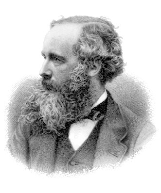
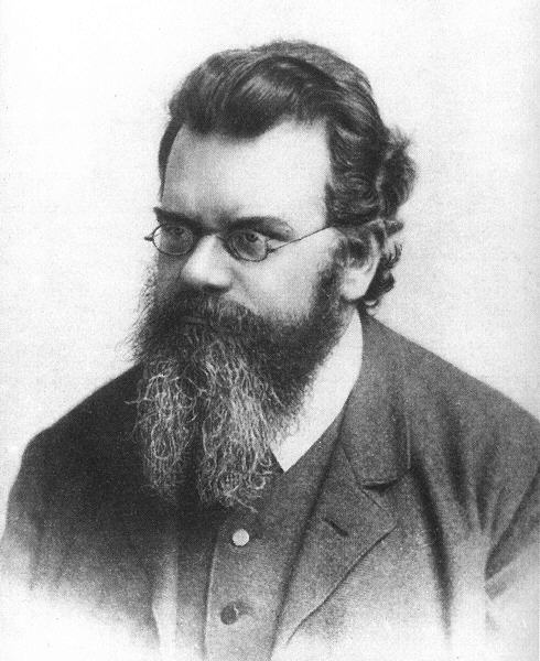
Figure: James Clerk Maxwell (1831–1879), Ludwig Boltzmann (1844–1906), Josiah Willard Gibbs (1839–1903). After Clausius the account becomes statistical: components of velocity, then occupation of energy, then free energy.
Clausius gave a macroscopic balance. Maxwell, Boltzmann and Gibbs give a microscopic count of the same \(S\). Maxwell’s first move is the velocity distribution: each Cartesian component is Gaussian, because the kinetic energy is quadratic. That quadratic is the energy whose expectation we will split as \(U=F+TS\).
Maxwell–Boltzmann: Components Versus Speed
Write the joint density on Cartesian velocities as isotropic, \[\begin{align} f(\mathbf{v}) = \left(\frac{m}{2\pi kT}\right)^{3/2} \exp\Bigl(-\frac{m|\mathbf{v}|^2}{2kT}\Bigr). \end{align}\] Each marginal \(f(v_x)\) is Gaussian. Change to spherical coordinates with \(v=|\mathbf{v}|\) and solid angle \(\Omega\). Probability conservation uses the volume element \(d^3v = v^2\,dv\,d\Omega\). Integrating over angles (\(\int d\Omega = 4\pi\)) gives the Maxwell speed distribution \[\begin{align} f(v) = 4\pi\left(\frac{m}{2\pi kT}\right)^{3/2} v^2\,e^{-mv^2/2kT}, \qquad v\ge 0. \end{align}\] The factor \(v^2\) is the Jacobian of the change of variables — the density of states of spherical shells in velocity space. Calling ``Maxwell–Boltzmann’’ Gaussian is correct for a component and wrong for speed.
\[ f(v_x)=\sqrt{\tfrac{m}{2\pi kT}}\,e^{-mv_x^2/2kT} \qquad\text{versus}\qquad f(v)\propto v^2\,e^{-mv^2/2kT} \]
The Gibbs–Boltzmann Distribution
Name the object and fix the formula. The MaxEnt derivation that earns these weights is a separate step: deriving the occupation from Lagrange multipliers before Shannon \(H\) and Jaynes would put the cart before the horse.
Write the equilibrium occupation of a discrete system with energies \(\{E_i\}\) as \[ p_i = \frac{e^{-\beta E_i}}{Z(\beta)}, \qquad Z(\beta)=\sum_j e^{-\beta E_j}. \] Physicists call \(p_i\) the Boltzmann distribution (or Boltzmann weights) and, for a system exchanging energy with a bath at fixed \(T\), the Gibbs distribution or canonical ensemble. The three names point at the same formula. The normalisation \(Z(\beta)\) is the partition function. Its logarithm \(\log Z(\beta)\) is the cumulant generating function for the energy under this exponential family: derivatives of \(\log Z\) recover the mean energy, the variance (heat capacity, up to factors of \(\beta\)), and higher cumulants. That generating-function reading is why \(Z\) is more than a normalisation constant.
Figure: Occupation of a two-state system as coldness increases. At low \(\beta\) both states are populated; at high \(\beta\) the ground state dominates.
The Gibbs–Boltzmann occupation is not only a statement about gases and magnets. Hopfield networks (Hopfield, 1982) assign an energy to every binary configuration of a recurrent net and treat recall as a descent toward low-energy states — equilibrium statistics are again Gibbs. Ackley, Hinton and Sejnowski (Ackley et al., 1985) made the weights of that energy learnable: a Boltzmann machine is an undirected model whose distribution over configurations is exactly \(p(s)\propto e^{-E(s)/T}\). The 2024 Nobel Prize in Physics, awarded to John Hopfield and Geoffrey Hinton, recognised that physical-systems reading of computation and learning. Name the lineage so the formula does not feel confined to nineteenth-century heat baths; do not divert into training algorithms.
Coldness and Temperature
The Boltzmann occupation can be written in two ways, \[ p_i = \frac{e^{-E_i/k_B T}}{Z} = \frac{e^{-\beta E_i}}{Z}, \qquad \beta = \frac{1}{k_B T}. \] The mathematics is the same, but the emphasis is different.
\(T\) is the variable of the bath. It is what a thermometer reports, and it is the intensive parameter in the Helmholtz accounting \(F = U - TS\). In that representation energy comes first and entropy is the correction: \(TS\) is the cut the second law takes from \(U\).
\(\beta\) is coldness. It is the variable conjugate to energy. In that representation entropy comes first: you maximise \(S\) (or write a generating function in \(\beta\)) and energy is the constraint. Temperature is then a derived reading, \(T = 1/k_B\beta = (\partial S/\partial U)^{-1}\).
We will use both. Weeks 1–2 keep \(T\) in view so the bath is familiar, and they already compute in \(\beta\) because that is the natural argument of \(Z\). Week 5 makes the \(\beta\)-first order honest: the Lagrange multiplier on a mean-energy constraint is coldness, and it is the natural parameter of the exponential family. Weeks 6–7 then treat \(\beta\) as a coordinate on that family. A student who still hears \(\beta\) as ``one over the thermometer’’ will miss why the geometry is written in those coordinates.
Free Energy Decomposition
Once the Gibbs occupation \[ p(x)=\frac{e^{-\beta E(x)}}{Z},\qquad Z=\sum_x e^{-\beta E(x)} \] is given, we can derive the macroscopic formulae that characterise the gas. They come to us from Helmholtz. We can compute them through the expectation of that occupation of the given energies, taken at equilibrium. The relationship between energy and probability is \(p_i\propto e^{-\beta E_i}\). Here we will identify the “inner energy” or “total energy” with \(\left\langle E\right\rangle\) and read off \(F=U-TS\). \(Z\) is German: it comes from Boltzmann, the sum of states, Summe der Zustände. That is why it is \(Z\), because it is a sum. If the system were continuous, a Gaussian, \(Z\) would be an integral.
Start from the occupation and take the logarithm, \[ \log p(x)=-\beta E(x)-\log Z. \] Note that nothing statistical has happened here, this is an identity for every probability that is a member of the exponential family, which in physics we think of as the Gibbs distribution. It’s valid for every configuration \(x\) that the Gibbs distribution supports. If we solve for the energy of that configuration we can restore temperature through recognising that \(\beta=1/(k_BT)\), \[ E(x)=-k_BT\log p(x)-k_BT\log Z. \] Note that the first term on the right (the surprisal multiplied by the temperature and Boltzmann’s constant) still depends on \(x\). The second does not: \(-k_BT\log Z\) is a property of the whole ensemble, not of a particular microstate.
At equilibrium the macroscopic inner energy can be related to the expectation of the microscopic score under the same distribution, \[ U\equiv\left\langle E\right\rangle=\sum_x p(x)\,E(x). \] This is where the ensemble is entering in physics. The ensemble that comes to us from Boltzmann, Maxwell, Gibbs, and Einstein. The idea is that the system is not in one configuration. When we coarse-grain this room we are not going to look at the actual energy of every particle. There are of order \(10^{23}\) of them; at that scale the variance around the expectation does not show. That expected energy becomes, at this scale, the total energy of the gas in the room. The index \(i\) is the space — discrete energy levels, which is one of the challenges Boltzmann received: what is this discrete space? That is where the phase-volume arguments come from. We will just assume it is discrete; an expectation is a sum or an integral. Substitute the identity for \(E(x)\), \[\begin{align} U &= \sum_x p(x)\bigl(-k_BT\log p(x)-k_BT\log Z\bigr) \nonumber\\ &= -k_BT\sum_x p(x)\log p(x) - k_BT\log Z. \end{align}\] The second term comes out of the sum because \(\log Z\) does not depend on \(x\), and \(\sum_x p(x)=1\).
The two remaining pieces already have names. The configuration-independent term is the Helmholtz free energy, \[ F=-k_BT\log Z, \] it is often known as the “free energy” or “available energy.” It is the energy that we can use for work. The average of \(-\log p\) is the dimensionless Shannon functional \(H=-\sum_x p(x)\log p(x)\). Multiplying by Boltzmann’s constant produces physical entropy, \(S=k_B H\), with units of energy per degree. Then \[ U=F+TS\qquad\text{or}\qquad F=U-TS. \] Helmholtz originally wrote \(A=U-TS\), with \(A\) for Arbeit, the work still available. This module uses \(F\) for the same quantity, because week 5 needs \(A(\boldsymbol{\theta})\) for the log-partition of an exponential family. But Helmholtz’s \(A\) and our \(F\) are the same object; \(U\) is the inner energy \(\left\langle E\right\rangle\), not a free energy. The fact that they are different is down to energy that is stored as entropy. It’s in this term that we can find Black’s latent heat.
From the physics and thermodynamics perspective \(U\) is the energy in the system, \(TS\) is the “cut” that entropy takes from that total energy. It is tied up in the uncertainty of the occupation, unavailable as work. Then \(F\) is what the thermodynamic bath still allows you to do. Given the Gibbs occupation, the macroscopic split \(F=U-TS\) is an identity.
The point of the derivation, boarded, is that inner energy is composed of the entropy plus the available energy. Entropy is now your bookkeeping device for why you cannot get all the work back out of the heat. You can convert all your work into heat and produce the inner energy with your motion. Then the motion is going in different directions. The energy is still there at the particle level. Maxwell’s demon is an attempt to reverse that by seeing where the particles are. The scale we have just written assumes an ensemble. Dive into the ensemble and play with it, and you cross levels of coarse graining. That is easy to do in modelling, and it is what goes on in a lot of Maxwell’s-demon arguments. It is not always clear at which point you are allowed to cross. Week 4 is the treatment; here it is the warning.
Watch the signs on the board. Boltzmann’s constant is of order \(10^{-23}\,\mathrm{J\,K}^{-1}\). There is a \(10^{-23}\) scaling on these numbers, and then of order \(10^{23}\) particles, so you get back to joules. The units of \(k_B\) are joules per kelvin — joules per degree. \(S=k_B H\) takes a dimensionless functional of a probability and converts it into the units we speak about. If you think of \(H\) as the more fundamental object, coldness \(\beta\) is the more natural parameter than \(T\). The reason we usually write it the other way around is that it was discovered in Clausius’s way: energy first, then entropy times temperature.
The \(T\)-first reading puts energy first and treats entropy as a correction. The \(\beta\)-first reading treats \(\log Z\) as a generating function: \(U=-\partial_\beta\log Z\) and \(S=\beta(U-F)\), which we compute from \(Z\) later. Both are the identity just derived. Later we will derive the occupation from MaxEnt and identify \(\beta\) as the Lagrange multiplier on the mean-energy constraint; until then the occupation is given, and we are reading it.
If you have a process whose entropy has not changed, inner energy and available energy are the same. That is a reversible system: you have not taken work and converted it into inner energy. Along a reversible path the heat relation is \(\mathrm{d}Q_{\mathrm{rev}}=T\,\mathrm{d}S\), or \(\mathrm{d}S=k_B\beta\,\mathrm{d}Q_{\mathrm{rev}}\). It comes from \(\mathrm{d}U=T\,\mathrm{d}S-p\,\mathrm{d}V\), not from the Helmholtz split. The thing they were measuring the flow of, when they talked about conservation, was entropy. That is the caloric they thought was conserved. If the entropy is conserved you are looking at a reversible system, which is what Carnot was trying to look at, and why his engine is the most efficient you can be.
A short history-of-science aside, boarded before the algebra. A lot of the practice of science in this period — what we might call engineering — is in Birmingham, Glasgow, Aberdeen, driven by application. Late nineteenth century, a rising capability in Germany. After the Great Exhibition of 1851 there was a royal commission to ask why Oxford and Cambridge had contributed so little. The result of that inquiry was the Cavendish Laboratory (1870) and the Natural Sciences Tripos. Maxwell is the scientist this thread is heading towards; we skip him for a moment.
Figure: \(U\), \(S\), and \(F\) for the Worksheet 1 three-state system (\(k_B=1\)). The dashed curve is \(-\log Z/\beta\); it sits on \(F\), which is the identity just derived.
The Worksheet 1 three-state system, \(E\in\{0,1,3\}\), is a numerical check of the same algebra with \(k_B=1\). Compute \(p_i=e^{-\beta E_i}/Z\), then \(U=\sum_i p_i E_i\) and \(S=-\sum_i p_i\log p_i\). The two expressions for free energy, \(F=U-S/\beta\) and \(F=-\log Z/\beta\), overlie. If they do not, the signs in the derivation are wrong.
import numpy as npdef gibbs_thermo(energies, beta):
"""U, S, F from a discrete Gibbs occupation ($k_B=1$)."""
e = np.asarray(energies, dtype=float)
weights = np.exp(-beta * e)
Z = weights.sum()
p = weights / Z
U = np.sum(p * e)
S = -np.sum(p * np.log(p))
F = -np.log(Z) / beta
return U, S, F, U - S / beta
U, S, F, F_from_US = gibbs_thermo([0.0, 1.0, 3.0], beta=1.0)
U, S, F, F_from_USAs Taught: Helmholtz on the Board
As taught on 27 October the Helmholtz algebra came immediately after the break, on the visualiser, before the Clausius slides. Paper went round first. A short history-of-science aside sat there too: after the Great Exhibition a royal commission asked why Oxford and Cambridge were not at the heart of the industrial work; the Cavendish Laboratory and the Natural Sciences Tripos are part of that answer (Cavendish, 1870). The Maxwell–Boltzmann and Gibbs slide decks were not opened first. The occupation from last week was already in the room; the job was to write it properly, \[ p_i = \frac{e^{-\beta E_i}}{Z},\qquad Z=\sum_i e^{-\beta E_i}. \] \(Z\) is German: sum of states, Summe der Zustände. Take the logarithm, take the expectation. Inner energy \(U\) is composed of an entropy term and an available-energy term in \(\log Z\). Watch the signs on the board. Surprisal is \(-\log p\).
A student asked why the exponential. Equilibrium. Another asked what \(\log Z\) is. Available energy: the work you can get out. The \(T\)–\(S\) square and the four-stroke as its implementation come next. Once the bookkeeping is in view, the Industrial Revolution is an information revolution.
Maxwell’s demon enters here as a preview, not as Week 4. You can convert all the work into heat. You cannot get all the heat back as work, because the motion is now going in different directions. The energy is still there at the particle level. The demon is an attempt to reverse that by seeing where the particles are. The scale we have just written assumes an ensemble. Dive into the ensemble and play with it, and you cross levels of coarse graining. That is easy to do in modelling. Week 4 is where the ledger is resolved; today is the warning.
The Carnot Cycle on \(T\)-\(S\)
A reversible engine is the most efficient you can be, such an engine is what Carnot studied. Along a reversible path \(\mathrm{d}Q_{\mathrm{rev}}=T\,\mathrm{d}S\), so the heat they treated as flowing with the mill is temperature times an entropy transfer. When they talked about heat flow and conservation, what they were actually measuring the flow of was entropy. This was the source of the caloric that they believed to be conserved. The ideal Carnot cycle makes that visible. It can be drawn on a temperature-entropy diagram as a square. That square is our picture, not his. Before drawing it, it is worth hearing what he actually asked.
Figure: Carnot’s own plate, 1824. Cylinder \(ab\), piston \(cd\), body \(A\) the furnace, body \(B\) the refrigerator. This is the mill as he drew it: not a waterwheel, a piston and two reservoirs. Vectorised from Réflexions sur la puissance motrice du feu (Wikimedia Commons, public domain).
We have already seen the mill: caloric falls from a hot body to a cold one, and the same caloric arrives at the bottom. His own plate is not a waterwheel. It is a cylinder and a movable piston, and two bodies, \(A\) and \(B\), held at different temperatures. The waterfall lives in the text, not in the figure (Carnot, 1824).
The sentence is careful. The motive power of a waterfall depends on its height and on the quantity of the liquid. The motive power of heat depends on the quantity of caloric and on what he will call the height of its fall — the difference of temperature between the bodies exchanging it. In a waterfall the work is exactly proportional to the difference of level. In the fall of caloric, he says, the motive power undoubtedly increases with the difference of temperature — but he does not know whether it is proportional. Would the same quantity of caloric falling from \(100^\circ\) to \(50^\circ\) furnish more or less motive power than the same caloric falling from \(50^\circ\) to zero? That is his question. Sit with it before the square appears. The square is our answer, not his. He identified the fall, and the reversible ceiling. He did not write \(W=\Delta T\times\Delta S\).
Figure: The same cycle twice. Left: a water mill on height against mass of water. Fill the bucket at the top, let it descend, empty it, return the empty bucket. The water is not consumed; the work is \(g\,\Delta h\,\Delta m\). Right: a reversible heat engine on \(T\) against \(S\). The conserved quantity in the reversible model is what we now call entropy. The vertical brace is Carnot’s fall — the difference between the reservoirs — not the downward stroke of the working body.
If you take the mill seriously as a cycle, it is already a rectangle. Fill the bucket at the top: mass comes in at height \(h_h\). The loaded bucket descends, the shaft turns. Empty at the bottom. Return the empty bucket. The water is not consumed. The work is \(g\,\Delta h\,\Delta m\).
Replace height by temperature and mass of water by entropy, and you have the \(T\)–\(S\) square. The conserved quantity in the reversible model is what we now call entropy. That is an interpretation of his caloric, not a claim that he had already discovered it without naming it. Falk reads Clausius’s entropy as a resurrection of caloric; Meyn draws the mill as this rectangle. Historians are not unanimous, and they should not be: the identification is a reading of the reversible model, not a reconstruction of what was in his head. What we can say is narrower. Once the transferred quantity is entropy and the height is thermodynamic temperature, the product is exactly the area, and proportionality is no longer a question. For a computer scientist this is a beautiful example of how choosing the right state variable turns a complicated process into simple geometry.
Figure: The ideal Carnot cycle on a temperature-entropy (\(T\)-\(S\)) diagram is a square. Heat is taken in along the top (\(T\) constant, \(S\) increasing) and rejected along the bottom. The two vertical legs are adiabatic: the working body changes temperature without exchanging entropy. The work extracted is the area, \(\Delta T\times\Delta S\).
You start at some temperature. In the Carnot cycle the temperature stays constant while the entropy increases: that is the expansion of the system, the increasing volume is the opening of the piston.1 Then the system cools — an isolated expansion, entropy holding. Once it has cooled, the entropy comes slowly back down, temperature staying the same: the contraction, heat rejected to the cold bath. That cold rejection is what Watt’s condenser is doing: it is the bottom of the mill, not the cooling stroke itself. Then you compress in isolation, the steam heats, and you have a square. This is the ideal engine. It is not how Carnot described it, but it is what he was describing.
On the visualiser I drew the two temperature changes as rapid, almost instantaneous. In the ideal cycle they need not be. They are adiabatic: thermally isolated, reversible expansions and compressions. No heat crosses the boundary, so entropy of the working body holds, and the temperature changes because the volume does. The entropy changes, by contrast, have to happen in contact with a bath. Do them too fast and you are no longer isothermal: compression would heat the system and expansion would cool it, and you have left the square.
\(\Delta T\) is the difference between the two temperatures and \(\Delta S\) the difference between the two entropies. The energy extracted on the cycle is \(\Delta T\times\Delta S\).
Figure: Two annotations that are easy to conflate. The vertical brace is Carnot’s fall of caloric: entropy is taken in at \(T_h\) and given up at \(T_c\). The right-hand leg is not that fall. It is an isolated expansion of the working body; no heat crosses, entropy holds, temperature drops.
It is easy to look at the square and take the downward stroke for the fall. That leg is where the working substance cools by expansion, with no heat transfer. Carnot’s fall is the difference between the temperatures at which entropy enters and leaves, across the whole cycle. The mill turns because caloric moves from \(A\) to \(B\), not because the piston is dropping.
He gives a concrete steam-engine example. A boiler at about \(160^\circ\mathrm{C}\), a condenser at about \(40^\circ\mathrm{C}\): a fall of caloric of \(120^\circ\). Combustion could furnish a much larger fall, a thousand degrees or more, and ordinary engines used only a modest part of it. That was his engineering point: look after the height. The modern reading, which he did not write, puts those on an absolute scale, \(T_h = 433\,\mathrm{K}\), \(T_c = 313\,\mathrm{K}\), and the ceiling is \(1-T_c/T_h\), a little under twenty-eight percent. The analogy suggested quantity of caloric times temperature fall. The \(T\)–\(S\) square tells us how that product arises, once the transferred quantity is entropy and temperature is thermodynamic temperature.
Figure: A real engine between the same reservoirs, with the same entropy swing, does not shrink the square. It still visits the top-right and the bottom-left. Heat is not taken in along the whole top, nor rejected along the whole bottom, so those two corners are cut off. The remaining area over the square is the efficiency.
In a motor-car engine the same loop is a four-stroke: ignition, piston down, exhaust, compression. This is known as the Otto cycle. But this is the mechanism behind the theory, or one possible mechanism. What the theory says is that the maximum energy you can get out is the area of the square.
The inner loop is easy to draw wrongly. You do not scale the square down. The fall is still \(T_h\) to \(T_c\), and the entropy change of the working body is still \(S_c\) to \(S_h\): those are known. So the top-right corner stays, and the bottom-left stays. What you lose is the other two. Heat does not go in isothermally along the whole top, nor come out along the whole bottom, and the area that remains, over the square, is the efficiency of the engine.
As an undergraduate mechanical engineer one learns these diagrams without anyone saying that the energy is stored in probability, or that this is the form of what entropy is. When you realise that the engine is at the heart of the industrial revolution and that it’s really converting entropy into work, then there is an argument that at its heart even the Industrial Revolution is an information revolution. That is, of course, if you accept the interpretation of entropy as information.
Figure: The same Carnot cycle on a \(p\)-\(V\) diagram. The hot and cold legs follow isotherms \(pV=\mathrm{const}\); the isolated cool and isolated heat follow adiabats, which are steeper. The enclosed area is still the work, \(\oint p\,\mathrm{d}V\), but you cannot read \(\Delta T\times\Delta S\) off it by eye.
The other way these things are drawn is as pressure-volume diagrams. You can draw the same stages as the \(T\)-\(S\) diagram, but they no longer look like straight lines. That’s because isothermal on this chart is a constraint on \(pV\) due to the relationship between pressure and volume (\(pV = nRT\) for an ideal gas). This makes it not so easy to read off what energy has been extracted because it’s the area inside the shape still, but the area is no longer a square.
But as a reminder, we are imposing a modern perspective on how Carnot thought about it. Recall his thinking was that it was more like a mill: a waterfall from which we are extracting energy. He did not talk about entropy. He was interested in change in temperature as being equivalent to height change. The \(p\)–\(V\) chart is Clapeyron’s language; the square is ours. The mill is his.
Two Sides of the Same Coin
We have just derived \(F=U-TS\) from the Gibbs occupation, with inner energy \(U=\left\langle E\right\rangle\). Helmholtz free energy is what remains after entropy’s cut. That identity is the whole of the LO1 payload. It is also why two research programmes that sound opposed are not. Welling, Lu and Holdijk’s Generative AI and Stochastic Thermodynamics was published this year. Its subtitle is A Tale of Free Energies (Welling et al., 2026). If that book had a slogan, it would be close to free energy is all you need. If this course had a slogan, it would be entropy is all you need. They are two sides of the same coin, and the coin is inner energy.
GAIST explores the shared mathematics of generative models and nonequilibrium thermodynamics. The mathematics is broadly the same; the philosophy is not. Their Chapter 3 is the Helmholtz split we have just done. Their Chapter 5 will identify variational free energy with the ELBO: inference as heat, learning as work. We will meet that identification in week 5 as a correspondence, not as a collapse of Shannon, Boltzmann and Jaynes into one theory. Read GAIST by chapter, not cover to cover. Callen remains the undergraduate thermodynamics. The motivations of this course — perpetual motion, the human bandwidth constraint — are not in that book.
Karl Friston’s free-energy principle treats the same variational free energy as an account of brains and of action: perception as inference that lowers a bound on surprise (Friston-free10?). Under a trial distribution \(q\) the functional is again \(U[q]-TS[q]\), which is Helmholtz’s split with the occupation replaced by \(q\). That is why it belongs in this lecture, and why it does not get a derivation today. We stay with entropy. Entropy is the cut that forbids perpetual motion. Free energy is what you can still do once that cut is taken. Inner energy is what you started with. Three names, one identity.
Preview: Shannon, Jaynes, Wiener
As taught this was the close, after Clausius, not the entropy-game slides. Shannon and Jaynes reuse the functional form for what might be said to be a different job. The argument of the course is to push those jobs back together when we return to Maxwell’s demon. Coldness is the more natural parameter when entropy is the thing you believe; Boltzmann’s constant is a scale in front of entropy.
Shannon is discrete. Wiener is continuous. Wiener never drops the mechanism. Shannon, you just say it is a probability. That is the no-go versus mechanism contrast from Week 1, now sitting on the information side. Week 4 and Week 5 are the treatments. Today is the hook.
The entropy game and MacKay’s weighing problem were named at 10:05 as the overflow: if the heat story ran, we would do them next week. They ran. They were not given on 27 October. They now open Week 4 after Quiz 2.
After Helmholtz: Not Reached
The physics story arrived at \(F=U-TS\). The information reading that Week 2 did not reach — guessing, MacKay’s weighing problem, and die coarse-graining — was named at 10:05 on 27 October and deferred at 10:33 and again at 11:56. Those slides now open Week 4 after Quiz 2, and they are the setup for Maxwell’s demon: the box as a group, the being who looks inside. Do not keep a second copy here.
Define This Week
The information game, MacKay and grouping open Week 4 after Quiz 2.
After This Lecture
Worksheet 2 (due start of lecture 4) presses whether Shannon \(H\) and Boltzmann \(S\) are the same object or a metaphor. Next week there is a class test — Quiz 2 — even though the webpage on 27 October said there was not. After the quiz: questions, MacKay, grouping, the missing measure, then Maxwell’s demon as compartments and two ledgers. The resolution families are Worksheet 3. Shannon / Jaynes / Wiener were previewed today.
Machine Review
A language-model review of the published notes for the L172 Week 3 session (27 October 2026). It is not assessed. Unlike the Week 2 review, it works from the written notes only, not the recording.
The Helmholtz derivation is correct, and the Worksheet 1 three-state check holds. The history serves the argument better than in Week 2. However, it has a cluster of dating and attribution errors. The title promises Shannon entropy, which the session did not deliver.
Fact check
Errors to fix
- Kelvin’s statement attributed to Clausius. “No cyclic engine converts the heat of a single bath entirely into work” is Thomson’s 1851 form. Clausius’s form is the cold-to-hot statement, made explicit in 1854.
- Clausius “without a notion of conservation of energy.” Helmholtz’s Über die Erhaltung der Kraft is 1847. Clausius’s 1850 first law, which introduces \(U\), is conservation of energy applied to heat. The lecture builds to “Helmholtz \(F=U-TS\)” but never mentions Helmholtz’s 1847 paper or his 1882 free-energy lecture. Adding both would fix the claim and give the payload its own history.
- Bernoulli “with momentum.” This contradicts Lecture 2, which credits Bernoulli with conservation of energy. Both are partly right: the kinetic chapter gets pressure from impacts (momentum), while the flow results use vis viva. Say which is meant.
- Helmholtz’s symbol. The notes say Helmholtz wrote \(A\), for Arbeit. The sources tie that to convention instead: IUPAC recommends the symbol \(A\) from the German word Arbeit, while physics also uses \(F\). From the reviewer’s own knowledge, and not checked against the 1882 original, Helmholtz used \(F\). If so, the justification “we use \(F\) instead of Helmholtz’s \(A\)” is backwards.
- “Shannon is always discrete.” Part III of the 1948 paper treats continuous sources, differential entropy, entropy power and the Gaussian channel (reviewer’s own knowledge). Lecture 2 itself teaches differential entropy. The Shannon/Wiener contrast should be about mechanism, not discreteness. The claim appears in both the Clausius section and the Preview.
- Caloric theory dated after Clapeyron. The notes say that after Clapeyron’s 1834 paper “people form what becomes known as the caloric theory of heat.” Caloric (Lavoisier’s calorique, 1789) predates Carnot. The Rumford section itself says caloric was already in Lavoisier’s table.
- Lavoisier and Laplace. There are three slips in one paragraph (reviewer’s own knowledge):
- Lavoisier’s 1789 list of elements is his own, building on the 1787 nomenclature with Guyton de Morveau, Berthollet and Fourcroy. Laplace was not a co-author.
- Oxygen was not “previously phlogiston.” Phlogiston was the theory that Lavoisier’s oxygen overturned; Priestley had called the gas “dephlogisticated air.”
- Napoleon made Laplace a count in 1806. The Restoration made him a marquis.
- Watt timeline. The Lap Engine was built by Boulton and Watt in 1788, not in the late 1770s or early 1780s. The first commercial Boulton & Watt engines ran in 1776 (reviewer’s own knowledge). That is about eleven years after the 1765 separate condenser, not “twenty-five to thirty years.”
- Newcomen. The cold water was injected into the cylinder, not sprayed onto it.
- Steam turbine efficiency. “A modern steam turbine is about sixty percent” is wrong. Steam-cycle power stations reach roughly \(35\)–\(47\%\); about \(60\%\) is a combined-cycle gas plant (reviewer’s own knowledge).
- The Cambridge aside. The Natural Sciences Tripos did not come out of the Great Exhibition. It was an immediate result of the earlier Royal Commission on the University, established in 1851, and physics was only included in it in 1873. The Duke of Devonshire’s offer came in October 1870, and the Laboratory was formally inaugurated on 16 June 1874. So “Cavendish (1870)” is the offer date, not the founding.
- Gremlins. The word does not date from the First World War. It was RAF slang among pilots in Malta, the Middle East and India in the 1920s, first printed in 1929; claims of a First World War origin have no print evidence. It was popularised in the Second World War.
- Four-stroke. The notes give the strokes as ignition, piston down, exhaust, compression. They are intake, compression, power and exhaust. The Otto cycle is also not “the same loop” as Carnot’s. Its ideal is two adiabats and two constant-volume legs, which is not a square on \(T\)–\(S\).
- Black’s timing. Four and a half times a fifteen-minute heat-up is about \(68\) minutes, not “an hour and a quarter” (that would be five times). The \(810\) figure uses \(4.5\).
Overstated or needs hedging
- “F is the energy we can use for work.” What bounds the work at constant \(T\) is \(-\Delta F\), not \(F\). \(F\) itself depends on the energy zero. The same applies to the answer “log \(Z\) is available energy.”
- “If entropy has not changed, inner energy and available energy are the same.” At fixed \(T\), \(\Delta S=0\) gives \(\Delta F=\Delta U\). It does not give \(F=U\).
- “That is the caloric they thought was conserved.” The Free Energy section states this as fact. The \(T\)–\(S\) section correctly hedges it as Falk’s reading. Use the hedge in both places.
- The real-engine \(T\)–\(S\) figure. The ratio of the real loop’s area to the Carnot square is a second-law (relative) efficiency, not “the efficiency”; thermal efficiency is \(W/Q_h\). A process that is not quasi-static also has no well-defined \(T\)–\(S\) path, so the cut-corner picture is schematic and should say so.
- “Why the exponential? Equilibrium.” As given, this answer leaves the occupation an unexplained postulate. The standard system-plus-reservoir argument derives the Boltzmann factor from the heat bath alone by expanding the bath’s log-multiplicity in energy. It needs no Shannon or MaxEnt, so it respects the lecture’s own ordering rule.
- ELBO. The ELBO is the negative of the variational free energy. “Identify variational free energy with the ELBO” needs the sign.
- Black’s latent heat of fusion.
- \(143\)–\(144\) Fahrenheit degrees is the modern value. Black’s own estimate is usually quoted near \(140\) (reviewer’s own knowledge, not checked).
- “\(80^\circ\mathrm{C}\)” should read “\(80\) Celsius degrees.” The paragraph’s own point is that this is not a temperature.
- Watt and high pressure. Watt’s opposition, and the extension of his patent to 1800, held back high-pressure work. “His patent covered engines that were not high-pressure” is muddled.
- Thomson “independently.” His 1851 paper credits Clausius with priority, so independence is Thomson’s own claim (reviewer’s own knowledge). Also, Thomson was \(23\) when the 1848 paper was read in June.
- Disclosure. Neil Lawrence’s endorsement appears among the book’s blurbs. A one-line disclosure would help where the course recommends Welling, Lu and Holdijk.
Checked and correct
- The Helmholtz derivation. \(\log p=-\beta E-\log Z\); \(U=F+TS\); \(F=-k_BT\log Z\); \(S=k_B H\).
- The Worksheet 1 three-state system. At \(\beta=1\) with \(E\in\{0,1,3\}\): \(U\approx 0.365\), \(S\approx 0.714\), and \(F\approx -0.349\) by both routes.
- Statistical-mechanics results. The Maxwell speed density and its \(v^2\) Jacobian; \(\log Z\) as the cumulant generating function; \(T=(\partial S/\partial U)^{-1}\).
- Carnot cycle results. Work equals the area \(\Delta T\cdot\Delta S\). \(1-313/433\approx 27.7\%\). Adiabats are steeper than isotherms on \(p\)–\(V\).
- Thomson 1848. The characteristic property as stated, infinite cold at \(-\infty\), and \(-273\) coming from the air coefficient.
- Joule. The British Association meeting at Cambridge in 1845, the figure of \(890\), and \(772.692\) ft·lb in 1850.
- Other historical details.
- Rumford’s 1798 timings, and the equal heat capacities of chips and solid metal.
- Carnot: the \(600\) copies, and death from cholera in 1832.
- Clapeyron, 1834.
- Clausius 1850, 1854 and 1865, including τροπή.
- The Fahrenheit and Celsius fixed points.
- Machine-learning lineage. Hopfield (1982), Ackley, Hinton and Sejnowski (1985), and the 2024 Nobel Prize.
- Welling, Lu and Holdijk now verifiable. The book is a 307-page Cambridge University Press title, dated 31 July 2026. Its epilogue is titled “Unification: free energy is all you need,” so the slogan the lecture attributes to it is literally the book’s own.
The review did not check Carnot’s \(160^\circ\mathrm{C}\) / \(40^\circ\mathrm{C}\) example, the Thurston page numbers, Meyn (2024), the cohort marks, or the comments on model behaviour.
Learning objectives
The notes call Helmholtz “the LO1 payload” but never state LO1.
Strengths:
- The payload is the right one. It is a single identity, derived rather than asserted, and checked numerically on the Worksheet 1 three-state system. It is also tied back to latent heat and the Carnot square. “Derive \(F=U-TS\) from the Gibbs occupation and verify it numerically” is a measurable objective.
- The history carries the argument. Each figure supplies one piece: heat as a quantity, the limit, non-conservation, the ratio scale, the state function.
- The Worksheet feedback is specific and usable. The see-saw and rat-holing patterns are concrete and actionable.
- It fills the Week 2 gap. Carnot and Clausius are now taught properly. That was the Week 2 review’s main objection.
Problems:
- The title does not match the content. The Shannon material in “Free Energy and Shannon Entropy” is a two-paragraph preview, and the axioms are parked. Either rename the lecture or teach the content.
- The carry-over is compounding. The info game, MacKay and the die example went from Week 2 to Week 3, and now to Week 4. HMC, which Week 2 promised for Week 3, has gone to parking.
- “Define This Week” lists only deferrals, with nothing to define.
- Week 4 now holds a quiz, MacKay, grouping, the missing measure and Maxwell’s demon.
- Something should be cut explicitly rather than left to drift.
- Opinion and settled result are still blurred in places. “The Industrial Revolution is an information revolution” is properly flagged as conditional on reading entropy as information. Do the same for “\(\beta\) is the more natural parameter” and the Shannon/Wiener mechanism contrast.
- The examinable version is unclear. Students need to know which week’s notes hold the examinable version of deferred material.
Editorial
- Unresolved citation keys. Nine render as “()”: Rumford-friction98, Thomson-absolute48, Thomson-dynamical51, Joule-equivalent45, Joule-equivalent50, Clausius-motive50, Clausius-equivalence54, Clausius-entropy65 and Friston-free10. “(Cavendish, 1870)” is also missing from the references.
- A missing item. “Black \(\to\) \(\to\) Helmholtz” has a gap in the sequence.
- Duplicated passages.
- The Maxwell’s demon preview appears twice.
- “You can convert all your work into heat” appears three times.
- The Shannon-discrete / Wiener-continuous passage appears twice.
- The “As Taught” section repeats the derivation section.
- An internal path.
_lamd/parking.mdappears in the student notes and means nothing to students. - Typos. “After Waterloo Lazare he was driven into exile”; “with a short hollow cylinder is turned.”
Sources
- Lecture 3
- Lecture 2
- Wikipedia, Kelvin (absolute scales)
- Chang and Yi, Thomson on absolute temperature, Annals of Science
- Science Museum Group, Lap Engine
- Wikipedia, Lap Engine
- Wikipedia, Helmholtz free energy
- Schweitzer, Welling, Lu and Holdijk (contents)
- Schweitzer, Welling, Lu and Holdijk (endorsements)
- CavMag, The birth of the Cavendish Laboratory
- Cavendish Laboratory, Our history
- Sevier, Founding of the Cavendish Laboratory
- Wikipedia, Gremlin
Further Reading
The mill analogy: motive power of heat compared to a waterfall of Carnot (1824)
The 1848 absolute scale: equal mill-degrees, ice still zero; \(-273^\circ\) is the air thermometer, not his bottom of (Thomson-absolute48?)
The 1845 letter: paddle wheel shown at the British Association, Cambridge; equivalent still scattered around 817 foot-pounds of (Joule-equivalent45?)
The 1850 Phil. Trans. paper: \(772\) foot-pounds; the settled equivalent of (Joule-equivalent50?)
The 1850 paper: two laws, Carnot’s limit without conserved heat of (Clausius-motive50?)
The 1865 memoir: \(\mathrm{d}S = \mathrm{d}Q_{\mathrm{rev}}/T\), and the name entropy of (Clausius-entropy65?)
The 1851 dynamical theory: Joule accepted; Thomson’s form of the second law. The ratio scale with a bottom is 1854, with Joule of (Thomson-dynamical51?)
Boltzmann machines (optional colour) of Ackley et al. (1985)
Hopfield networks (optional colour) of Hopfield (1982)
The waterfall: quantity of liquid, height of the fall; he does not yet know if the work is proportional (Thurston pp.~60–61) of Carnot (1824)
Entropy as a resurrection of caloric of Falk (1985)
The mill drawn as a rectangle; caloric in the reversible model read as entropy of Meyn (2024)
A tale of free energies: the Helmholtz split is Ch.~3; we stay with entropy of Welling et al. (2026)
The free-energy principle: the same split, used as a theory of brains of (Friston-free10?)
Chapters 1–4 of Callen (1985)
Chapters 5–6 of Callen (1985)
Thanks!
For more information on these subjects and more you might want to check the following resources.
- company: Trent AI
- book: The Atomic Human
- twitter: @lawrennd
- podcast: The Talking Machines
- newspaper: Guardian Profile Page
- blog: http://inverseprobability.com
References
Focussing on volume increase, normally we would expect increasing volume to cause cooling, but in a heat engine if we increase the volume slowly enough, heat can flow from a heat bath to the cylinder and it stays at constant temperature. The energy is flowing in from the heat bath.↩︎