

Week 2: Ensemble, Entropy, and Embodiment
[jupyter][google colab][reveal][edit]
Abstract:
Worksheet 1 is due and the session starts with Quiz 1 (probability and Week 1 energy seeds). We reopen Laplace’s ``molecule of air’’ as an anachronism, state Bernoulli’s kinetic assumptions, and introduce the statistical ensemble as coarse-graining. Then Hydrodynamica, the entropy bridge (no-go versus prescription; common distributions; continuous / relative entropy named), and embodiment as bandwidth (The Atomic Human). As delivered we stop there. Week 3 is the heat thread through Helmholtz, then MacKay / grouping.
Worksheet 1 is due at the start of this session. The slot is 10:05–11:55 (110 minutes, not 120). Quiz 1 occupies the first ten minutes from 10:05. After the quiz: Laplace’s molecule, Bernoulli / Hydrodynamica, ensemble as coarse-graining. Entropy bridge (distributions; continuous entropy and relative entropy / KL named) sat after the break; embodiment (Atomic Human) was the last ten minutes. As delivered we stop at embodiment — overrun to 12:00. Week 3 is the heat thread (Black through Helmholtz), then the unfinished info game / MacKay / die coarse-graining. Do not derive the occupation from MaxEnt today — that is week 5.
This Session
Time plan (as delivered 20 October 2026). Clocks from the Panopto recording (00:00 ≈ 10:00) plus the transcript. The slot is 10:05–11:55 (110 minutes, not 120). Quiz silence is 10:08–10:18; the break ran 11:09–11:17 (spoken as five minutes, started late). Entropy review sat after the break; embodiment was the last ten minutes, not the whole second hour. Close overran five-to.
| Clock | Block |
|---|---|
| 10:05–10:18 | Quiz 1 (Moodle; briefing then ~10 minutes sitting) |
| 10:18–11:09 | Laplace molecule; Bernoulli / Hydrodynamica; ensemble / coarse-graining |
| 11:09–11:17 | Break |
| 11:17–11:50 | Entropy bridge; common distributions; continuous / KL named |
| 11:50–12:00 | Embodiment / bits as bandwidth (Atomic Human); flag Week 3 carry-over |
Quiz 1
Invigilated Moodle, own device, no notes, no network, no LLMs. Ten questions on last week’s probability review and the energy / Boltzmann seeds pressed in Worksheet 1. Hydrodynamica and the entropy bridge follow the quiz.
Class test timer: 10:05
From Daniel Bernoulli: Week 1 Carry-Over
Week 1 stopped at Daniel Bernoulli’s book, having already quoted Laplace on the curve of a molecule of air. We open by pressing how anachronistic that sounds once atoms are in dispute in Boltzmann’s century, then Bernoulli’s assumptions, then the ensemble as the coarse-grained answer to Laplace’s gremlin. Hydrodynamica, billiards, and the entropy bridge follow inside the same include; Gibbs–Boltzmann accounting waits for Week 3.
Laplace’s Molecule: an Anachronism?
How does that notion of entropy relate to our notion of information? This is a contested space. I am giving you my perspective; you will be able to explore whether it is contested in other works.
Laplace’s gremlin suggests that the curve of a simple molecule of air or vapour is regulated as certainly as a planetary orbit, the difference being our ignorance (Laplace, 1814). With some thought, this might sound anachronistic. He is writing in 1814. He predates atomic theory as physicists later understood it, and he predates the chemist’s molecule. So what is his notion of a molecule? He is saying that its motion is determined as a planet’s is.
Boltzmann, operating nearly a hundred years after Laplace, is trying to produce a molecular or atomic theory of matter, and that claim is disputed in his time. Other physicists disagree with him. In chemistry the story is quite different, because they have the periodic table. In physics the notion of a molecule is not there. Boltzmann takes his own life in 1906, and one of the reasons is thought to be his struggle to have the atomic theory accepted.
Einstein’s annus mirabilis is 1905. Special relativity and the photoelectric effect dominate the retelling, but one of the papers is on Brownian motion. He does not discover Brownian motion — that is Robert Brown, about fifty years earlier — but he writes stochastic differential equations to describe it. That is a molecular theory, in effect, and it is not validated by experiment for a couple of years. Boltzmann dies without his ideas being accepted. Energeticists such as Ostwald and positivists such as Mach treated atoms as optional or metaphysical. Only after Perrin’s experiments (1908–1909) did the molecular hypothesis become unavoidable for the mainstream. So why is Laplace, writing in 1814, already talking about molecules?
In early modern and Enlightenment usage, molecule often meant a minute body or corpuscle. It is the Newtonian residue of a particulate theory of matter, not yet a stoichiometrically defined chemical molecule of the late nineteenth century. Laplace is not citing Dalton, who comes from the chemical perspective. He is citing Newton, who has a corpuscular language.
The English translation we have says molecule. Perhaps it should be corpuscle. I do not know enough about the language and the history; that is an open question. The word is coming to us as a translation of French, and my supposition is that it enters English as a scientific word only once we have a chemical sense of it.
When we read old science we tend to project our modern context onto it, particularly if a translator has rendered molécule as molecule, where the contemporary English might have been corpuscle.
Laplace’s point in the Essai is epistemological: even if these air molecules followed a determined trajectory, we lack the data, the laws in usable form, and the computation to track it, so we turn to probability. The gremlin is still valid, because Laplace’s idea does carry through. That is our modern notion of how air is made up. The gremlin is ignorance of the particle’s path. It is not a claim that atoms were established. The ontological fight over whether those particles exist is yet to come. Why do we not perceive these molecules at particular scales? That is a property of coarse-graining in physics, and for me it is closely related to the way we abstract concepts in our intelligence.
Laplace’s perspective on air comes from Daniel Bernoulli, who preceded him by three-quarters of a century.
Hydrodynamica
When Laplace spoke of the curve of a simple molecule of air, he may well have been thinking of work from about seventy-five years earlier, bridging Newton to Laplace: Daniel Bernoulli (1700–1782), and Hydrodynamica.
People know the Bernoulli effect: constrict a flow, the fluid speeds up, the pressure changes — the cartoon of what lets planes fly. The diagrams draw particle lines around a wing and say that this particle goes around the top, that one around the bottom, and the upper one has to go faster because the path is longer. Why does it not simply arrive late? Fluid dynamics is hard to have a good sense of because we are working across different coarse grains.
Daniel Bernoulli, I think, is the first person to take a corpuscular model of a fluid and treat the particles as sitting in a little element, as we do in a modern discretisation. He effectively uses conservation of energy, which is striking, because Newton had treated momentum. I think it is Huygens who does conservation of energy.
He was the son of Johann Bernoulli — uncle Jacob was the other giant of that generation; Johann’s other student was Euler. Johann treated his son with remarkable hostility: he took the work, published it under his own name, and backdated it. That is why Daniel ended up in St Petersburg, at a time when Russia was founding universities, and Euler joined him there for a while. He produced a large body of work; this one was read an enormous amount. He is writing in Latin, in 1738, already treating a gas as many tiny bodies in motion.
Figure: Daniel Bernoulli’s Hydrodynamica published in 1738. It was one of the first works to use the idea of conservation of energy. It used Newton’s laws to predict the behaviour of gases.
Daniel Bernoulli described a kinetic theory of gases, but it was not until 170 years later that these ideas were verified, after Einstein had proposed a model of Brownian motion which Jean Baptiste Perrin confirmed experimentally.
Figure: Daniel Bernoulli’s chapter on the kinetic theory of gases, for a review on the context of this chapter see Mikhailov (n.d.). For 1738 this is extraordinary thinking. The notion of kinetic theory of gases would not become fully accepted in Physics until 1908 when a model of Einstein’s was verified by Jean Baptiste Perrin.
What Bernoulli Assumes
Daniel Bernoulli’s kinetic chapter in Hydrodynamica (Mikhailov, n.d.) asks what pressure is if air is a swarm of particles. The modelling assumptions are severe and productive:Conservation of mechanical effect (energy in later language) lets him relate microscopic motion to macroscopic push. That is an extraordinary claim for 1738. It is also an idealisation: real molecules attract and vibrate; Bernoulli’s gas is a coarse mechanical cartoon chosen so that Newton’s laws have something to act on.
Even at the birth of kinetic theory, the useful object is not the full list of paths. Bernoulli averages. He is not tracking Laplace’s curve for every particle — he predates Laplace — but he is summarising a swarm of motion. Individual trajectories are discarded, and what remains is a mechanical story for pressure. That pressure is macroscopic and measurable: when a vessel explodes, it is the pressure we are talking about, and that is a function of particles hitting the walls. There is a great deal of energy stored in that.
The statistical physicists who follow — Maxwell, Boltzmann, Gibbs — will turn that averaging into an explicit probability over microstates. The billiard simulation is Bernoulli’s assumption made visible; the Shannon entropy of the velocity histogram is already a coarse-grained proxy for how much velocity detail we are keeping.
I think Bernoulli is probably the first person to start doing this move that we are going to see throughout the course. It sits at the heart of entropy, and at the heart of intelligence. The move is coarse-graining.
Entropy Billiards
Figure: Bernoulli’s simple kinetic models of gases assume that the molecules of air operate like billiard balls. Without small variations in the initial conditions they would never bump into each other. The displayed entropy is the Shannon entropy of the observed discrete velocity histogram (a coarse-grained proxy, not the differential entropy of a Gaussian, and not full thermodynamic entropy).
Velocity Histogram
import numpy as npp = np.random.randn(10000, 1)
xlim = [-4, 4]
x = np.linspace(xlim[0], xlim[1], 200)
y = 1/np.sqrt(2*np.pi)*np.exp(-0.5*x*x)Another important figure for Cambridge was the first to derive the probability distribution that results from small balls banging together in this manner. In doing so, James Clerk Maxwell founded the field of statistical physics.
Figure: Maxwell (1831–1879): each Cartesian velocity component of an ideal-gas particle is Gaussian. Speed \(v=|\mathbf{v}|\) is not — it picks up a \(v^2\) Jacobian.
The distribution of speed and velocities are Maxwell–Boltzmann physics. Confusing them is easy because textbooks say “Maxwell–Boltzmann distribution” for either object. The geometric factor \(v^2\) is a change of variables. The transformation is also revealing. Continuous entropy is not invariant under the transformation, but relative entropy (or KL divergence) is. We will use this example to help explain why differential entropy is needed in the continuous case.
From Paths to an Ensemble
We ignore some portion of the detail and summarise it with its macroscopic statistics. In physics, that is what Gibbs called the ensemble.
A microstate is the curve of the simple molecule of air — the positions and velocities of all the particles. A macrostate is how we summarise it: particle number, volume, energy, temperature, pressure. An ensemble is the probability of the microstates compatible with the macrostate.
Bernoulli never looked at it as probabilities. He looked at it as we might do in fluid flow today, drawing a box around a subsection of the flow. Gibbs comes a little after Boltzmann. I do not think Boltzmann used the term, but Boltzmann was doing the same thing.
This maps directly into the way we model in machine learning. If I say the noise is Gaussian, I am doing the same thing: I look at it with its mean and its variance. When we include noise in a machine learning model, we are allowing the model to abstract. We are allowing it to ignore some of the underlying process. In physics they typically prove that that is the case. In machine learning we assume it and try to fit the model.
Physicists distinguish extensive from intensive. An extensive property is a macrostate property that scales with the size of the system. An intensive property does not. Temperature is intensive. \(N\) is extensive. Volume scales extensively. Energy tends to increase with the system.
Is entropy intensive or extensive? One route is that we can calculate one thermodynamic quantity from another, so they must scale in roughly the same way. Another is that entropy increases as I increase the state space. If I have \(N\) independent variables from the same distribution, the total entropy is \(N\) times each variable’s entropy. Entropy therefore scales extensively. That is also why, later, \(TS\) having units of energy tells us that entropy must be extensive.
I think coarse-graining sits at the heart of entropy and at the heart of intelligence. Bernoulli does not track Laplace’s curve for every particle. He summarises a swarm of motion. In that summarisation we lose information, because we are no longer tracking everything that is going on, but we convert the summary into something operational on the level above.
That move is common in physics. As we go into the material, into the atom, these summarisations occur multiple times. In advanced physics we meet renormalisation. Why do objects pop out at certain scales? Why are there levels at which particles appear? That is at the heart of what is going on in physics.
My argument is that something similar happens in intelligence. Which part of this is a table, and which part is not? We think about causal relationships between the table and the piece of paper; about what is a mug and what is not. What is the relationship between the physical summarisation going on here, and the summarisation we perform when we interact with the world? For me that is one of the critical things about our intelligence: how we abstract objects.
My preferred example is a hurricane. A colleague, Niall Robinson, worked at the Met Office on large-scale simulations and on data coming out of Navier–Stokes. He had to define what a hurricane is. There is no variable “hurricane” in Navier–Stokes. There is a load of particles moving around. To identify a hurricane in the simulation you write a list of things: wind speeds above a threshold, the storm in a certain place. You take our sense of a hurricane and convert it into criteria.
From the equations’ perspective there is not an object. It is air moving around and interacting with water and land. I think we would all agree that hurricanes exist. That is an abstraction. When we talk about a fluid we are doing the same thing. It is really a bunch of molecules moving around together; then we think of its properties at a higher level.
A hurricane is comparatively clean — Niall could define it quite well — unlike a chair. People struggled for years in computer vision to write logical rules that define a chair. It is not as sharp as gas, liquid, solid.
What this abstraction buys us is that we can summarise the gas in the room by its temperature, pressure and volume, instead of by the movement of every particle. Similarly, I can talk about what we do when a hurricane is approaching New Orleans. I do not have to talk about all the bits and pieces moving in the hurricane. I can make decisions at a different level of abstraction. Operating at the right level of abstraction seems to me a key part of intelligent decision making.
I will not mark you wrong for disagreeing. That claim is my speculation, not settled science. It is a route I find worth taking.
Some of this table’s properties are clearly macrostates of the system, such as its volume and its temperature. Then there are other things where the relationship is no longer so tight. That is where my notion of abstraction breaks away from the kinetic story. We cannot summarise the table as some simple distribution. There are correlations inside it. There is structure — chains within the wood — complex things going on in the states of the table that are not true of the gas around us. The table is not in a maximum-entropy state, in that sense.
The gas around us is noise. There is energy in what is going on there, but there is no correlation or structure in it. That is why we can summarise it by the temperature, the pressure and the volume. Independence is also a property of maximum entropy. If there were correlation, it would not be maximum entropy.
We can look at the same system and coarse-grain at different levels. That is again what physicists are doing when they increase the energy in a particle accelerator. They are looking at things that are around us, but they are increasing the energy.
When I histogram the bins, I am keeping some of the velocity detail and discarding the rest. Different bin widths would have given a different entropy. That choice is a coarse-graining choice, and it affects the entropies we see.
Thermodynamics is a coarse-graining choice to keep the temperature, the volume and the pressure. The merit of that choice is that we know the form of the residual we are losing: it is a maximum entropy. I do not think that is quite true of the residual if I am histogramming.
The uncertainty we are calling entropy lives at that chosen grain. When we make these choices, we are discarding something and creating entropy. A choice of discretisation triggers an entropy loss.
This came up with a student, Francisco Vargas, working on Schrödinger’s bridge. He had a sampling approach, the Schrödinger–Föllmer sampler, billed as an exact sampler. In Bayesian inference we want to sample from the posterior, and normally we do that approximately. His sampler was exact only if the diffusion it was based on ran continuously. There is a nonlinear diffusion that has to be solved numerically. As soon as you discretise that diffusion, you produce entropy, and the sample is no longer exact. The coarser the discretisation, the more entropy you produce, and the worse the approximation.
What stops us discretising infinitely? Assume a numerical mathematician has solved stability for us. Why would we not discretise infinitely? Why, when we do weather, do we not go down to millimetres? UK weather predictions currently use cells of about 800 metres. Halve the grid size and you quadruple the computational cost. Discretising more means we have to make more computations.
If I coarse-grain more finely, I discard less entropy, but I have to compute more. Is that trade-off fundamental, or a coincidence? In the thermodynamics of engines we claim that the trade-off is fundamental. An engine that stays closer to equilibrium can be more efficient; if it moves slowly, it is more efficient and less powerful.
There is an entropic argument, and then there is an argument about how you are doing it. That is also what I claimed is problematic in Maxwell’s demon: one argument is entropic, and then there is another — how is the demon doing it?
What follows historically is the bookkeeping that makes the ensemble usable. Gibbs–Boltzmann occupation, free energy \(F=U-TS\), and the bath that justifies fixing \(T\) wait for the next lecture. The molecular hypothesis wins historically, but today we need the abstraction: we replace ignorance of the path with a distribution on the set of paths, and the cost of that move is how much uncertainty the macro description throws away.
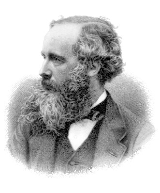
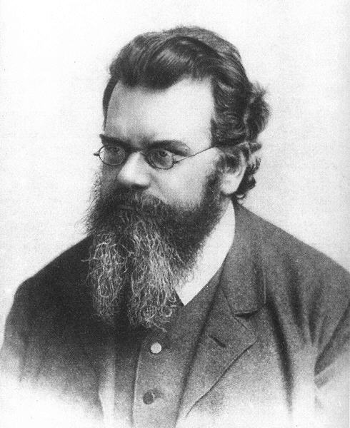
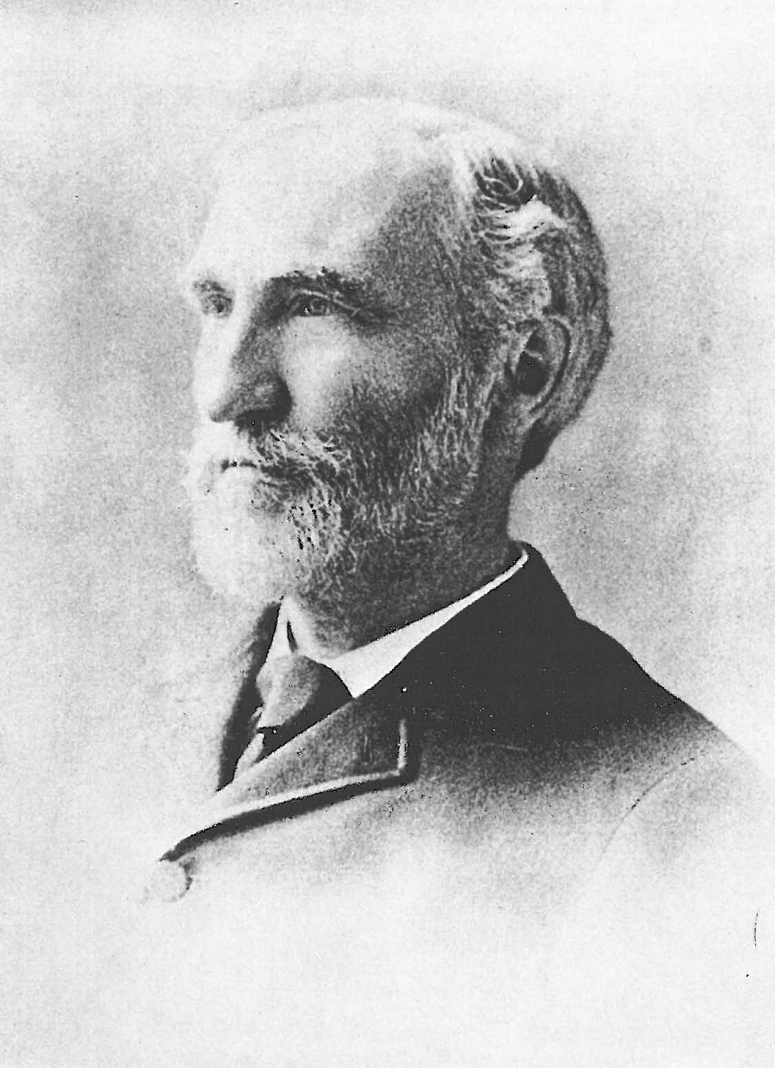
Figure: James Clerk Maxwell (1831-1879), Ludwig Boltzmann (1844-1906) Josiah Willard Gibbs (1839-1903)
Many of the ideas of early statistical physicists were rejected by physicists who did not believe in the notion of a molecule. When Boltzmann was writing, it was still unclear whether heat was a fluid — it has fluid-like properties because it seems to flow. The Graz paper is a foundation paper in the kinetic theory of gases. It was a radical change of perspective.
Max Planck took the work up early. Boltzmann had persistent trouble with German physicists, including Mach. Planck was a champion of his. The reason Planck talks about scientific theories proceeding one funeral at a time is that this perspective was so radical. You can see why the existing community resisted it. A lot of physics is about fields, continuous fields — still is today — and particle theories were obnoxious to that clean, continuous picture.
Boltzmann took his own life in 1906, two years before the molecular picture became widely accepted. Whether the controversy caused that is contested. Some biographies tie the suicide to the fight over atoms; the Stanford Encyclopedia of Philosophy treats that causal story as a myth and points instead to depression and declining health.
Figure: Boltzmann’s paper Boltzmann (n.d.) which introduced the relationship between entropy and probability. A translation with notes is available in Sharp and Matschinsky (2015).
The important point about the uncertainty being represented here is that it is not genuine stochasticity, it is a lack of knowledge about the system. Maxwell, Boltzmann and Gibbs give us a description of the macrostate through a small set of parameters — volume, temperature and pressure — that are sufficient statistics for the gas, linked by an equation of state. They do not specify the microstate: which molecule is where, with which velocity. When we approximate the physical world we sit somewhere between the deterministic and purely stochastic worlds those scientists described.
One ongoing characteristic of people who study probability and uncertainty is the confidence with which they hold opinions about it. Arthur Eddington, then at the Cambridge Observatory rather than the Cavendish, expressed his support of the second law of thermodynamics (which Gibbs and Boltzmann made statistical: entropy increases almost always, not always) with an emphatic statement around page 74 of The Nature of the Physical World, in the chapters on the second law, not at the opening of the book (Eddington, 1929).
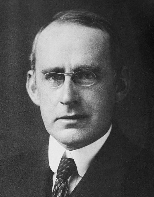
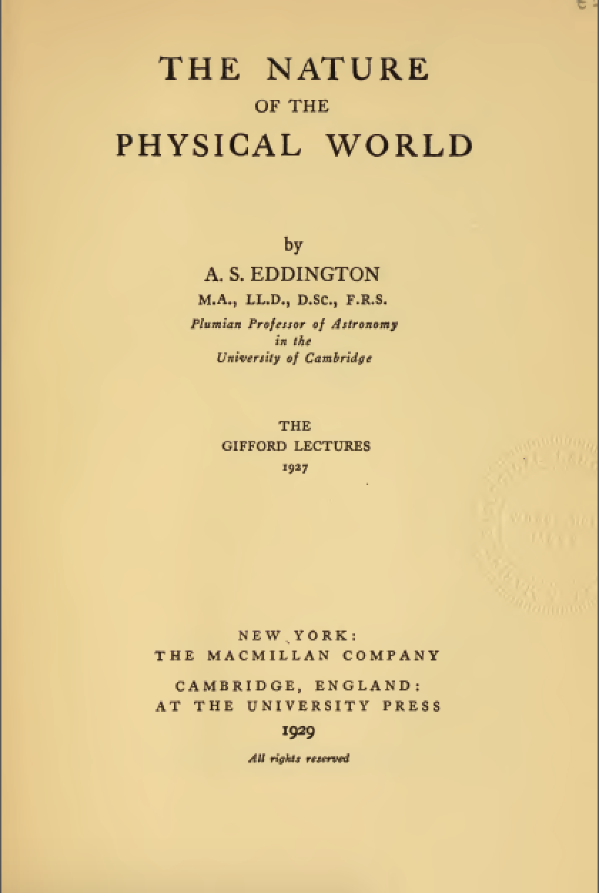
Figure: Eddington’s book on the Nature of the Physical World (Eddington, 1929)
The same Eddington dismissed the ideas of a young Chandrasekhar. Chandrasekhar had come from India to Cambridge; he was at Trinity, not the Cavendish. On 11 January 1935, at a public meeting of the Royal Astronomical Society, he presented the mass limit for a white dwarf. Beyond that limit the end state is a neutron star or a black hole — he did not use those names — not simply “a singularity.” Eddington carried his ideas too far. He humiliated Chandrasekhar in public. The documented remark is that there should be a law of Nature to prevent a star behaving in such an absurd way; “abomination” is a later paraphrase. Whether Eddington’s faith in the second law drove the dismissal is speculation; one account notes that he did not directly refute Chandrasekhar’s mathematics. Chandrasekhar was deeply upset, later received the Nobel prize for the work, and disliked the controversy that followed him. Accounts of the meeting: Universe Today, Southampton, The Stellar Graveyard, Flamsteed Astronomy Society.
Why would Eddington dislike the theory? All the mass of the universe ending up in black holes is not the maximum-entropy state. The maximum-entropy state is like the gas in this room: heat death. Chandrasekhar experienced the exchange as racially charged. That reading is understandable; it is not, on the evidence we have of Eddington — who was open across the First World War to German physicists — the best explanation. My belief is that he thought he saw the limit contradict the second law, and so he said to Chandrasekhar: that cannot happen.
That confuses mechanism with the law. Black holes evaporate: Hawking radiation. They do not stay in this state, but the evaporation takes a very long time. The second law still applies, as a slow leakage away from this concentration of mass. The better response would have been: the physics shows that this happens; I expect maximum entropy to apply in the long time; what is the mechanism through which this undoes itself?
I can believe in the second law of thermodynamics. I should not humiliate a student who comes up with a mechanism that initially seems to contradict it, because the two arguments work at different levels. Eddington would not have felt he was humiliating. He would have thought that he was teaching. There is a way of teaching, when you are a very senior physicist, that can be very damaging.
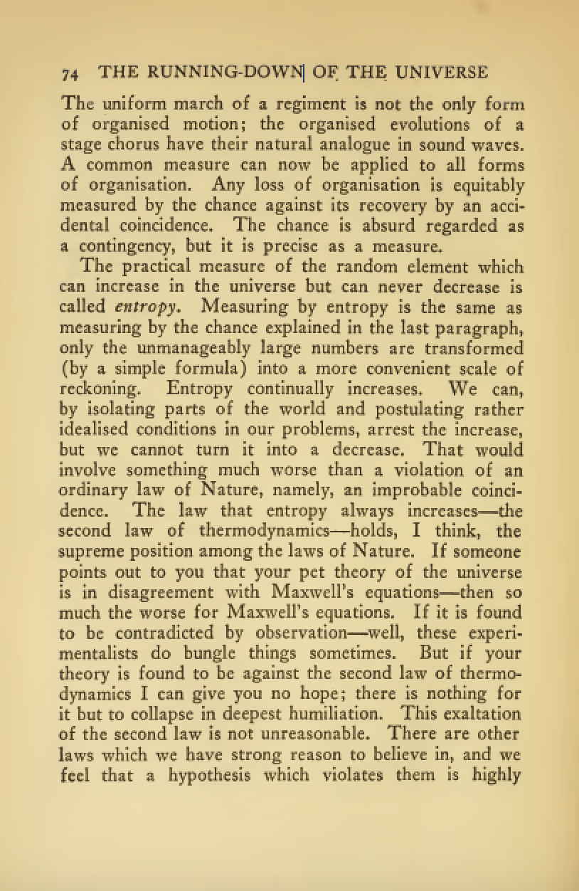
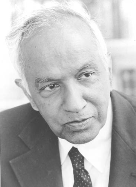
Figure: Chandrasekhar (1910-1995) derived the white-dwarf mass limit. Eddington dismissed the result at the RAS on 11 January 1935, humiliating a young scientist who would later receive a Nobel prize for the work.
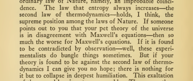
Figure: Eddington makes his feelings about the primacy of the second law clear (around p.74 of (Eddington, 1929), not the opening). Gibbs and Boltzmann made the law statistical: entropy increases almost always. A convenient extract is at Today in Science History.
The cropped quote is the one I paraphrase: if your theory contradicts Maxwell’s equations, so much for Maxwell’s equations; if it does not match experiment, well, experimentalists do bungle things at times; but if your theory contradicts the second law of thermodynamics, I have nothing but the deepest humiliation for you. The second law holds, he thinks, the supreme position amongst the laws of nature. Hawking radiation is the slow mechanism. Do not confuse teaching with humiliation.
Entropy Review
That last number is Shannon entropy in nats: \(H(p)=\mathbb{E}_{p}[-\log p(y)]=-\sum_y p(y)\log p(y)\). Same arithmetic under another name.
Under Shannon’s definition, entropy is dimensionless. It is the expectation of the negative log surprisal, \(-\left\langle\log P(y)\right\rangle\). In machine learning we might call that the energy or the objective function. It returns uncertainty as a single number.
That number has to compose correctly. If I am choosing to ensemble the gas in this room, someone outside is ensembling this room and the people in it, and someone on another planet is looking at us and summarising the whole planet, I would like the calculus of my entropy to work across that composition. As we coarse-grain, I would like entropy to reflect the loss that occurs at every grain.
That compositional property is one of the things that gives you this functional form. If it did not look like that, I could coarse-grain at this level, record my information loss, then coarse-grain at the level above, and the losses would be inconsistent. That is the mathematical motivation for the Shannon form. The information game and MacKay’s balance — the operational reading as fair yes/no questions — wait for week 3.
Entropy of Common Distributions
Shannon entropy is an expectation of surprisal: \(H=\mathbb{E}[-\log_2 P(X)]\). The right-hand panel makes that literal. We walk the same five families as the probability review — Bernoulli, binomial, Poisson, multinomial/categorical, Gaussian — so the entropy of each object sits next to the object itself.
Bernoulli Entropy
A Bernoulli(\(p\)) random variable takes values \(\{0,1\}\) with probabilities \(1-p\) and \(p\). Its Shannon entropy is the binary entropy \[ H(X) = -p\log_2 p - (1-p)\log_2(1-p) \] bits. The panels below show, for a fixed \(p\), the distribution, the pointwise surprisal \(-\log_2 P(x)\), and the summands \(-P(x)\log_2 P(x)\) whose total is \(H\).
Figure: Bernoulli(\(p=0.3\)). Left: the distribution. Middle: surprisal \(-\log_2 P(x)\). Right: the summands \(-P(x)\log_2 P(x)\); their total is the entropy \(H\).
Binomial Entropy
A Binomial(\(n,p\)) count is the sum of \(n\) i.i.d. Bernoulli trials. There is no elementary closed form for \(H\), but the same three-panel reading applies: plot \(P(k)\), plot \(-\log_2 P(k)\), and sum \(-P(k)\log_2 P(k)\). For large \(n\) a Gaussian approximation gives \(H\approx\tfrac12\log_2\bigl(2\pi e\, np(1-p)\bigr)\) bits.
Figure: Binomial(\(n=12\), \(p=0.4\)). The right-hand panel sums to \(H\); tails contribute little because \(P(k)\) is small even when surprisal is large.
Poisson Entropy
A Poisson(\(\lambda\)) distribution on the non-negative integers has \[ P(k)=\frac{\lambda^k e^{-\lambda}}{k!}. \] Entropy again has no elementary closed form; numerically \(H=\sum_k -P(k)\log_2 P(k)\). For large \(\lambda\), \(H\approx\tfrac12\log_2(2\pi e\lambda)\) bits.
Figure: Poisson(\(\lambda=4\)). Mid: surprisal rises in the tails. Right: the probability weight cuts those tails back, so \(H\) is dominated by the bulk.
Multinomial / Categorical Entropy
One draw from a multinomial (a categorical distribution) on \(K\) categories with probabilities \(\mathbf{p}=(p_1,\ldots,p_K)\) has entropy \[ H = -\sum_{k=1}^K p_k\log_2 p_k \] bits — exactly Shannon’s formula. The four-outcome table from the expectation example is already a categorical; we reuse those probabilities here.
Figure: The four-outcome distribution from the expectation example, now in bits. Right-hand summands total \(H\); category \(y=3\) is rarest (highest surprisal) but contributes modestly because \(P(3)\) is small.
For \(n\) i.i.d. categorical draws the joint entropy is \(nH\); the entropy of the count vector (the multinomial sufficient statistic) is smaller because many sequences share the same counts. Today we only need the single-draw / categorical case — it is Shannon’s sum in pure form.
Gaussian Differential Entropy
For a continuous density the same formal expression \[ h(X) = -\int p(y)\log_2 p(y)\,\mathrm{d}y \] is called differential entropy. It can be negative, and it is not invariant to rescaling of \(y\). For a univariate Gaussian \(\mathcal{N}(\mu,\sigma^2)\), \[ h = \tfrac12\log_2\bigl(2\pi e\sigma^2\bigr) \] bits. The panels below use the height example (\(\mu=1.7\), \(\sigma^2=0.0225\)): density, surprisal \(-\log_2 p(y)\), and the integrand \(-p(y)\log_2 p(y)\).
Figure: Univariate Gaussian (height example). Middle: \(-\log_2 p(y)\); dips below zero where the density exceeds \(1\). Right: the integrand whose integral is differential entropy \(h\).
We are not yet giving Shannon’s channel-capacity theorem, which many would say is the sophisticated piece of his work. Philosophically, this part of the construction is doing something else. It explicitly takes away mechanism. I am not sure that he highlighted this; it is the bit I want to keep. He does not say what your coding system has to be. He does not want to talk about your mechanism for doing the actual integral. He is saying: you are going to lose entropy if you discretise in that way.
When we go into the thermodynamic entropy I will tend to use \(S\) for the physical entropy and \(H\) for Shannon’s entropy.
Thermodynamic entropy \(S\) and Shannon \(H\) have a shared functional form. In equilibrium we can write \(S = k_B H\) when \(H\) is in nats. If \(H\) is computed in bits (\(\log_2\)), the conversion is \(S = k_B \ln 2 \cdot H\). Boltzmann’s constant is \(k_B = 1.380649 \times 10^{-23} \tfrac{\text{kg}\text{m}^2 }{\text{s}^2 \text{K}}\).
So there are two parts to a thermodynamic entropy, one is the uncertainty of a (discrete) distribution. The other translates that entropy into units of ‘work’ i.e. (\(\text{J} = \tfrac{\text{kg}\,\text{m}^2 }{\text{s}^2}\)) per Kelvin (\(\tfrac{\text{J}}{\text{K}}\)). Boltzmann’s constant makes entropy physical. When we multiply \(S\) by temperature \(T\) (in degrees Kelvin) we recover a term that has units of energy. That \(TS\) has units of energy is also why entropy must be extensive: if I have \(N\) independent copies, \(H\) scales with \(N\), and so does \(TS\).
I feel that this object is mathematically more fundamental than any notion of energy. You can imagine a world in which it is the other way round: you start by deriving entropy, and then you look at things in the other direction. Why is that not this world? Because no one can measure entropy. You do not measure it directly. There is no way, in an empirical science, that you would see this entropy production going on. You only start realising it is happening when you have missing quantities to explain. A physicist would say there is no way of measuring entropy directly — although we will look at situations where entropy reduction is immediate, as when I tell you the result of a coin toss and a reduction of one bit has occurred. That is coming because we know what the probabilities were.
But the dependence of entropy on the states of a distribution, or the probability across those states, also implies that there is a choice in terms of which states we consider. In classical mechanics we have states like position and velocity (or momentum). But quantum mechanics also leads to other properties of materials such as the spin of an electron. Choice of which variables you consider when computing e.g. the entropy of an electron, was referred to as the ‘“anthropomorphic” nature of entropy’ by Jaynes (1965). He credits this remark originally to Eugene Wigner. One example that Jaynes gives is thermodynamic steam tables.
If we work with a system of degrees of freedom, the experimental entropy is a function \(S_{0}(X_{1}\ldots X_{n})\) of \(n\) independent variables. But the system has any number of additional degrees of freedom \(X_{n + 1},\ X_{n + 2}\), etc. We have to understand that these additional degrees of freedom are not to be tampered with during the experiments on the \(n\) degrees of interest; otherwise one could easily produce apparent violations of the second law. Jaynes (1965) (my emphasis)
He goes on to give an example from entropy of steam (which is very important in the design of steam engines and power plants).
For example, the engineers have their “steam tables,” which give measured values of the entropy of superheated steam at various temperatures and pressures. But the H$_2$0 molecule has a large electric dipole moment; and so the entropy of steam depends appreciably on the electric field strength present. It must always be understood implicitly (because it is never stated explicitly) that this extra thermodynamic degree of freedom was not tampered with during the experiments on which the steam tables are based; which means, in this case, that the electric field was not inadvertently varied from one measurement to the next.
This leads him to a conclusion that is worth bearing in mind when we talk about the physical meaning of entropy. Once you have those steam tables, you can make a better steam engine or a better steam turbine. They were not measuring the entropy of the spin in the electrons, or whatever else is going on in the atomic physics, when they created the tables. That is what Jaynes means by anthropomorphic.
If I talk about the entropy of a die, you will probably assume I am talking about a fair die with six pips on it. You do not assume I am talking about the entropy of the underlying fabric of that die. So it is contextual. In physics they are trying to make sure that choice is valid in an objective way. In machine learning and AI that choice is subjective: it depends on who you are, what time frame you are operating over, what you are trying to achieve, what senses you have. From my perspective it makes no sense to talk about intelligence without this context — cuttlefish, crows, whether large language models have some form of embodiment because they have learnt it from us.
Recognition that the “entropy of a physical system” is not meaningful without further qualifications is important in clarifying many questions concerning irreversibility and the second law. For example, I have been asked several times whether, in my opinion, a biological system, say a cat, which converts inanimate food into a highly organized structure and behavior, represents a violation of the second law. The answer I always give is that, until we specify the set of parameters which define the thermodynamic state of the cat, no definite question has been asked!
Returning to the mathematical form of entropy, the fact that it is based on probability means that many of the properties of probability carry across to entropy. But the use of the logarithm means that they manifest as additions instead of multiplications.
For example the joint entropy of two variables, \[ H(X, Y) = - \sum_{X, Y} P(X, Y) \log P(X, Y), \] can be decomposed as the entropy of the marginal and the entropy of the conditional, \[ H(X, Y) = H(X \mid Y) + H(Y) \] where \[ H(X \mid Y) = - \sum_{X, Y} P(X, Y) \log P(X \mid Y) \] and \[ H(Y) = - \sum_{Y} P(Y) \log P(Y). \] This is known as the chain rule of entropy (Cover and Thomas, 1991). And it follows from the product rule.
The equivalent of Bayes’ rule is \[ H(Y \mid X) = H(X \mid Y) + H(Y) - H(X). \]
Entropy and Probability
I’ve spent most of my career in machine learning thinking about uncertainty, and very often that’s been through probability. For so-called “Bayesian” researchers, one of the most important texts is Ed Jaynes’s “Probability, the Logic of Science” (Jaynes, 2003), which has become almost akin to a religious text. However, alongside probability, and also in Jaynes’s work there’s been a recurring theme of entropy and information arising.
I started my PhD in 1996 at Aston University, but in 1998 moved to Cambridge, following my PhD supervisor who’d moved to Microsoft Research. I was excited because one of the most important researchers studying uncertainty in neural networks was based in Cambridge in the Cavendish lab. His name was David MacKay, and because there were no neural network researchers in the Computer Lab at the time I went to his group meetings. His group was called the inference group.
MacKay’s work had been inspired by Stephen Gull’s work in the MaxEnt, and his PhD thesis applied the Laplace approximation to uncertainty in neural networks — he did not introduce the approximation. I was excited to learn more. So you can imagine I was surprised and confused to see that David had become more interested in error correcting codes and information theory. Or at least that’s where his group’s focus had shifted. And one of the main mathematical objects underpinning these codes was entropy.
As a mechanical engineer, lacking the mathematical background of the physicists around me, I had to learn somewhat by osmosis. Chemical osmosis is driven by ionic gradients. Intellectual osmosis is driven by intriguing explanations.
A mechanical engineer needs to learn thermodynamics. I answered exams using tables that contained the entropy of superheated steam. I studied thermodynamics in my undergraduate degree at Southampton from a textbook by Rogers and Mayhew in the 1990s. It was the same textbook my father had studied from when he studied mechanical engineering in Sheffield in the 1960s.
So, I think this got me to thinking about a few things. What was the entropy of steam to do with the entropy of a communication code (if anything?). In the nearly three decades since those meetings I find I’ve been thinking about that for some time. And I notice that while my understanding of entropy has (I hope!) evolved, Rogers and Mayhew is still an assigned textbook for some thermodynamics courses https://library.buid.ac.ae/meng234.
Probability and entropy are tightly interlinked. And I’ve been increasingly thinking if entropy should really be the principal object we think about when considering uncertainty, not probability. I don’t know if I’m right, but the idea of this course is to share some of those ideas.
Why do I think entropy should be the principal object? Well there’s a funny thing about it that I can’t quite put my finger on, an aspect of entropy that has teased me for a while. And I’d like to explore that aspect in this course with you.
Here’s the problem with probability. Every time I specify a probability distribution, I need to specify all that happens. I don’t get to say that the distribution looks like a bell curve on the right, but I don’t know what’s going on on the left. I need my probability to both cover the things I’m interested in, and the things I might not be interested in. It feels like with probability I have to specify everything that’s going to happen.1 Entropy however is different. With entropy, it feels like I get to talk about what’s not going to happen. In information theory forms of entropy help us understand “no-go” areas, like the amount of information a channel is not going to carry per second … or at least an upper bound on the information that the channel will carry. In physics, the second law of thermodynamics helps us understand that perpetual motion won’t happen. It doesn’t tell us the mechanism by which a system will lose energy and eventually slow and stop. It doesn’t tell us when it will happen (unless we start looking at rates of energy to entropy conversion) it just tells us that it’s going to happen.
I find that intriguing.
But just because I find something intriguing it doesn’t make it true. So in some sense this will be a course about opinion. And it needs to be so. Because opinions about entropy vary. We’ll try and capture that variety as we go. But to try and bring some narrative coherence to the course, we will explore the variety through a narrative based on my opinion. That doesn’t make my opinion right, it just makes it the easiest way to deliver the course.
But why study entropy in Computer Science? Well, while we’re on the subject of opinion, and bear in mind I’m really a mechanical engineer, so don’t take my opinion too seriously. If there is any science in computer science, then it must be the science of how information evolves. The time it takes to process it and the transformations we can apply to it. But information theory is often absent from computer science courses. Why is that? Well because until now we have had to focus mainly on the techniques and tools we need to use to process data. On programming, on hardware implementation. On the mechanics of the information processing. Not the thermodynamics of the information processing. We have focussed on the mechanisms through which we transform information, not the fundamental rules by which it is transformed.
Today things are shifting rapidly, my community has developed tools that allow the computer to communicate directly in natural language with humans and program for them. We have finally created computer systems that can be driven by anyone through natural language, just as my mechanical engineering predecessors created cars that could be driven by anyone without having to have an understanding of how a connecting rod is connected to a crank shaft.
The field is changing rapidly. But students are being taught thermodynamics today from books that are the same as those it was taught from 60 years ago.
It’s my instinct that those books provide important theory that tell us about the limits of computing machines. Today there are many making promises about superintelligent AGI machines that do all we can do more rapidly and more capably. A world where cognitive decision making knows no bounds. This course is built on the following premise. That premise is that there will be bounds and that those bounds will be dictated by information theory. Or more precisely, the information dynamics of the system.
Just as thermodynamics tells us that there is no perpetual motion, I believe information dynamics will tell us that there are boundaries to the notion of superintelligence singularity. We won’t achieve those boundaries in this course, but we will provide a journey through the landscape of entropy in a way that may persuade you that these are interesting tools to seek those boundaries with.2
When modelling in practice, we often account for this with cost functions. There’s a funny thing about entropy too. One idea that will emerge across the course is the notion that probability tells us what a system will do. But entropy (somehow) tells us what a system won’t do. For example, we know that perpetual motion machines can’t exist because, by the second law of thermodynamics, they cause entropy to be produced. Kelvin and Clausius forbid extracting work from a single heat reservoir. A frictionless wheel could spin forever without violating the second law; what stops a real wheel is friction, which dumps organised motion into heat. The law forbids a machine that turns that heat back into organised work with nothing else changing. It doesn’t tell us the dynamics by which the spinning will stop. It doesn’t tell us when it will stop. It just tells us that we cannot have a perpetual-motion engine. If we had the probability distribution that described the system, that would tell us when the wheel was likely to stop. So somehow probability tells us what’s going to happen, whereas entropy tells us what’s not going to happen. We’ll explore this intuition as we go through the course, but it’s behind the idea why we might look to entropy to place limits on the performance of an intelligent system.
The second law of thermodynamics doesn’t tell you how to build an engine. Shannon’s capacity theorem doesn’t tell you how to construct a code. They tell you what’s not going to happen. This is common among entropies: they give you prohibition.
The Atomic Human
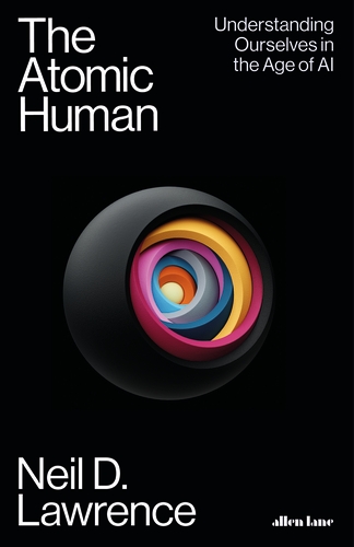
Figure: The Atomic Human (Lawrence, 2024).
There is one equation in the book, and it is accidental: \(E=mc^2\), because everyone knows it. The book is a way of looking at human intelligence. The main thing that is going on with our intelligence is its context. You cannot simply replicate our intelligence. You can emulate it, but you cannot replicate it, because it has a specific context.
The notion of the atomic human is this. Any capability I have, anything I do that we can measure, I believe we can probably get machines to emulate. We could get a machine to look at the measurement, optimise some parameters, and recreate it — if the thing I am doing, we can measure.
Then the question becomes: is the notion of artificial general intelligence valid? That is how the claim is usually framed, or superintelligence: a machine that is better in all these ways of measuring. This is a different way of looking at our intelligence.
I do not know how to define intelligence, but there is a process we can go through. It is equivalent to Democritus’s atoms — which, I presume, later inspired the corpuscles. If I cut this table in half, describe one half, cut the next piece in half, and keep going: can I do that forever, or do I reach a point where I cannot cut?
The Greek atomists, around 400 BC, said you reach a point where you cannot cut, and the world is made of those things. CERN chose to split the atom — but that just means we misnamed the atom. Below an atom you go to a quark. I do not think anyone can split that. There is some notion of something indivisible in the physical world.
The notion in The Atomic Human is the same idea in our cognitive landscape. Every time a machine does something that used to be unique to humans, it is slicing into us. Cut something away. Does that process go on forever, or is there a point at which it stops?
In a public-understanding talk I pause, and you have to find your own answers. Ask computer scientists, and some will say there is no point at which it stops, and humans disappear. I think that is a bleak answer. Ask other people, and they say there is a point at which it stops. They offer “true empathy,” or — one of the answers I return to — suffering. Another answer I return to, even though I am not religious, was “my relationship with God.” I think both these answers are informative. But I’m not saying there’s a single right answer. I’m saying it is a question anyone can ask, and you can ask yourself.
My specific answer is that the thing the machine cannot have is our weaknesses and our vulnerabilities, because they are intrinsic to us. I can emulate an entity. I can recreate my capabilities — anything I can score. The vulnerabilities and limitations I have are fundamental to us.
That limitation is one of the dominant reasons our intelligence is the way it is. Instead of dumping the contents of a computation, we have to turn these things into things other people might be able to relate to, in order to communicate very complex subjects.
The cultural landscape we sit in is something we constructed, so that I can, with very few bits of information, point to an idea that you already know and say: this is like this. Why that works remains something of a mystery. Why do analogies work? As you go deeper into it, I am not sure there is a derived principle. But they do work, and that is how we communicate. So much of our intelligence is about building up this world around us.
The notion of AGI, on this argument, does not survive. Unless you have that limitation embedded, it is not a general intelligence; it is specific to us and our context. You can emulate it, but it is not the same. I think the claim is empty.
My arguments on that are all based on Shannon’s bits. I set aside conversation about intelligence, and I asked: how much information is coming in over what time? That is why I think information is powerful in this space. We can see that the machine is already six orders of magnitude better off than us, just by the physics of it. The things we are seeing today are a consequence of that.
What has that got to do with information theory? Key among those limitations is one we are not going to treat in this course — I’d suggest death remains the domain of theology — but it is true: we are all going to die. The difference this course will focus on is what I think of as the embodiment factor: my ability to communicate versus my ability to compute, and yours as well.
That limitation is one of the dominant reasons our intelligence is the way it is. Instead of dumping the contents of a computation, I have to stand here and say: it is a bit like Boltzmann did this; here is another story of Gibbs; this person took his own life. I have to turn these things into things you might be able to relate to, in order to communicate very complex subjects. You might disagree about how well they worked today.
You do not lose marks for believing in AGI, superintelligence, and existential catastrophe. I think the claim is empty. The argument we will use in this course is Shannon’s bits.
Information and Embodiment
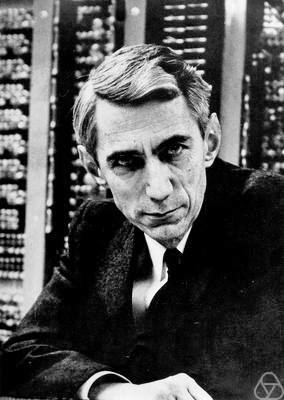
Figure: Claude Shannon (1916-2001)
| bits/min | billions | 2,000 |
| calculations/s | ~100 billion | a billion billion |
| embodiment | 20 minutes | ~billion years |
Figure: Embodiment factors are the ratio between our ability to compute and our ability to communicate. Relative to the machine we are also locked in. In the table we represent embodiment as the length of time it would take to communicate one second’s worth of computation. For computers it is a matter of minutes, but for a human, it is a matter of thousands of millions of years.
I am using voice, sound, to communicate with you. Those communications propagate at about 300 metres per second. The speed of light is about \(3\times 10^{8}\) metres per second — a million times larger than 300. If I had stood here and given this lecture by sending light waves instead of speaking, I would have gone a million times faster, even using the same mode of communication.
Now look at bits per minute. I am probably speaking at 150 words a minute. Shannon’s later paper on printed English estimated \(11.82\) bits per word from word frequencies (Zipf’s law, no context) (Shannon, 1951). That is the “\(\sim 12\) bits per word” figure; it is not from the 1948 paper. With context his estimates fall to around one bit per letter, so true word entropy is much lower. Using the crude \(12\) bits/word figure I am speaking to you at about \(2{,}000\) bits per minute, or about \(30\) bits per second. The “\(10\)–\(60\) bits/s” band is that same crude estimate at typical speaking rates Lawrence (2024), not Shannon’s context-conditioned entropy. Two machines on a gigabit link are not merely a million times faster than that. The difference in their communication rates, relative to us, is the difference between walking — one metre per second — and the speed of light.
Computationally our brain is very fast. The best estimates we have suggest you would need a very large computer to simulate it. If one computer wants to tell another computer everything it computed in one second, my estimate is that it would take about 20 minutes. For a human the ratio is far larger. At \(2{,}000\) bits per minute, a billion calculations per second would take about a year to talk out. The slogan in the table — around a billion years — needs around \(10^{18}\) calculations per second, a “billion billion.” That is an order-of-magnitude claim with those two assumptions stated, not a measured brain flop rate. I cannot access one second of neuron firings, and the computer cannot access it either.
We can talk about embodiment physically, in terms of what it means to touch something, and in terms of what it means to sense the world. This difference in our context, in what we are doing in our relationship with the world, is what defines our intelligence.
Shannon measured information in bits: one bit is the result of a fair coin toss. The \(\sim 12\) bits per English word figure is \(11.82\) bits/word from word frequencies in (Shannon, 1951), not the 1948 paper; it is a crude Zipf estimate, and with context the entropy per letter falls to around one bit. With typical speaking rates that crude figure gives \(\sim 10\)–\(60\) bits per second for human communication Lawrence (2024). Machines communicate orders of magnitude faster — the embodiment factor is the ratio between compute and that narrow channel.
As promised on 20 October, Week 3 was to take MacKay after the heat thread. As taught on 27 October the heat thread filled the slot. The information game, MacKay and grouping now open Week 4 after Quiz 2.
Define This Week
Interpret later: how entropy is understood today; equilibrium versus non-equilibrium; die grouping, Gibbs / \(F\), HMC, bath and Schottky (Week 3); the purely entropic Schottky reading (Week 8). Define-stage answer to “How was entropy discovered?”: Carnot on engines (1824); Clausius states the second law in the 1850s and coins the name entropy in 1865; Boltzmann and Gibbs give the statistical count; Shannon and Jaynes reuse \(H\) with different operational readings.
After This Lecture
Next week is the heat thread through Helmholtz, then MacKay / grouping. Shannon \(H\), \(Z\), KL, bath / Schottky are parked in Week 4 for sorting. Optional LLM probe: is free energy a constraint or a recipe? (after \(F\) is taught).
Machine Review
A language-model review of L172 Week 2 (20 October 2026), against the written notes as of 1 November 2026. It is not assessed. The original historical and technical errors in the notes have been absorbed.
Still open
- Figure caption versus table. The embodiment table cells say \(\sim\)billion years. The figure caption still says “thousands of millions of years” (
_ai/includes/embodiment-factors-celsius.md). - Questions page versus lecture. Questions still lists “Who were Carnot and Clausius, and what did each contribute?” as a Lecture 2 define item. The lecture file dropped that item; Week 3 taught the heat thread.
- Week 2 define items are still not measurable. “How was entropy discovered?” and “What are the information constraints on a human?” ask for recall.
- Other snippets, not this lecture.
_ai/includes/embodiment-factors-table.htmland_ai/includes/embodiment-factors-tedx.mdstill have the old “a billion” / “5 billion years” / “15 billion years” arithmetic.
Remaining fixes
- Align the embodiment figure caption with the table (“\(\sim\)billion years”).
- Move “Who were Carnot and Clausius ?” from Lecture 2 define to Lecture 3 on the Questions page.
Sources
Further Reading
- Chapter 1 of Lawrence (2024)
Thanks!
For more information on these subjects and more you might want to check the following resources.
- company: Trent AI
- book: The Atomic Human
- twitter: @lawrennd
- podcast: The Talking Machines
- newspaper: Guardian Profile Page
- blog: http://inverseprobability.com
References
That’s not strictly true because I can marginalise things I’m not interested in … but gives me a challenge of integrating over those variables which can lead to mathematical (or computational) headaches.↩︎
Fortunately, even if I’m totally wrong, the tools are widely deployed in a number of domains and your efforts in understanding them will bear fruit in one domain or another.↩︎