Ensemble, Entropy, and Embodiment
FW26, William Gates Building
This Session
- Quiz 1 (ten minutes)
- Laplace’s molecule → Bernoulli assumptions → ensemble as coarse-graining
- Hydrodynamica / entropy bridge (distributions; continuous / relative entropy named)
- Embodiment / bits as bandwidth (Atomic Human) — stop
- Next week: Black → Helmholtz, then MacKay / grouping
Quiz 1
- Device required; Moodle open
- No notes, no network, no LLMs
- Ten minutes
From Daniel Bernoulli: Week 1 Carry-Over
Laplace’s Molecule: an Anachronism?
Laplace spoke of “a simple molecule of air.” That sounds anachronistic once we meet Boltzmann.
- Laplace, Essai (1814): the curve of a molecule is as determined as a planet’s
- Boltzmann dies in 1906 still fighting atomists’ opponents
- Atoms / molecules were not settled science in the nineteenth century
“Molecule” Before Chemistry Won
Laplace is not citing Dalton. He is speaking Newton’s corpuscular language.
- French molécule: a small particle of matter, not yet the chemist’s molecule
- The kinetic idea is older than the chemical proof of atoms
- The gremlin is ignorance of that particle’s path, not a claim that atoms were established
Hydrodynamica
Daniel Bernoulli (1738) already treats a gas as many tiny bodies in motion.


What Bernoulli Assumes
Hydrodynamica (1738) already treats a gas as many tiny bodies in motion.
- Many corpuscles, small compared with the vessel
- Motion is swift and disordered; collisions transfer momentum
- Pressure on a wall is the rain of impacts, not a static push
- Idealisation: elastic billiard-like encounters, no lingering forces
Assumptions Are Already Coarse
Bernoulli does not track Laplace’s curve for every particle — he summarises a swarm.
- Individual trajectories are discarded
- What remains is a mechanical story for pressure
- Next: make the discarded detail a probability — the ensemble
Entropy Billiards
Velocity Histogram
Gaussian Components, Not Speed
The histogram above is one component \(v_x\). The Maxwell speed distribution is different, \(|v|\).
- Component \(v_x\): Gaussian (what we plotted)
- Speed \(v=|\mathbf{v}|\): \(f(v)\propto v^2 e^{-mv^2/2kT}\)
- Week 3: how that change of variables shifts continuous entropy
From Paths to an Ensemble
Laplace’s gremlin says we cannot follow every curve. The ensemble is how we live with that.
- Microstate: positions and velocities of all particles (Laplace’s curves)
- Macrostate: a few numbers — \(N\), \(V\), \(E\) or \(T\), \(P\)
- Ensemble: a probability over the microstates compatible with the macrostate
Extensive and Intensive
Some macrostate properties scale with the size of the system. Some do not.
- Extensive: \(N\), \(V\), energy — scale with the system
- Intensive: temperature — does not
- Entropy is extensive: \(N\) independent copies \(\Rightarrow\) \(N\) times the entropy
A Hurricane Is Not in the Equations
There is no variable “hurricane” in Navier–Stokes.
- Just air, water, land — particles moving around
- We still all agree hurricanes exist
- Right level of abstraction is how we decide
The Table Is Not Maximum Entropy
Some of a table’s properties look like macrostates. The rest is structure.
- Volume and temperature: gas-like summaries
- Grain, chains in the wood: correlations we are not throwing away
- The table is not in a maximum-entropy state
Coarse-Graining Is a Choice of Description
Temperature and pressure are sufficient statistics of the swarm
- Histogram bins: keep some velocity detail, discard the rest
- Thermodynamics: keep \(T\), \(V\), \(P\); discard which molecule was which
- The uncertainty we write as entropy lives at the chosen grain
Discretisation Produces Entropy
Finer grain: discard less entropy, compute more.
- Exact only if you track the continuous thing
- UK weather: cells of about 800 metres — why not a millimetre?
- Slow engines are more efficient and less powerful. Is that the same trade-off?
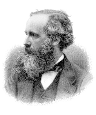
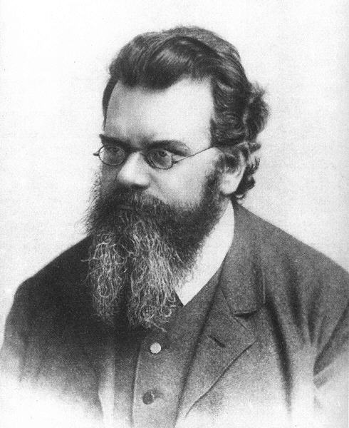
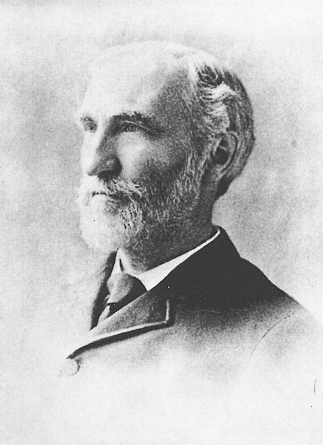
Bridge to Maxwell, Boltzmann, Gibbs
They turn Bernoulli’s swarm and Laplace’s ignorance into a calculus.
- Maxwell: velocity statistics of the ideal gas
- Boltzmann: \(S\) linked to probability over microstates
- Gibbs: ensembles as the systematic language

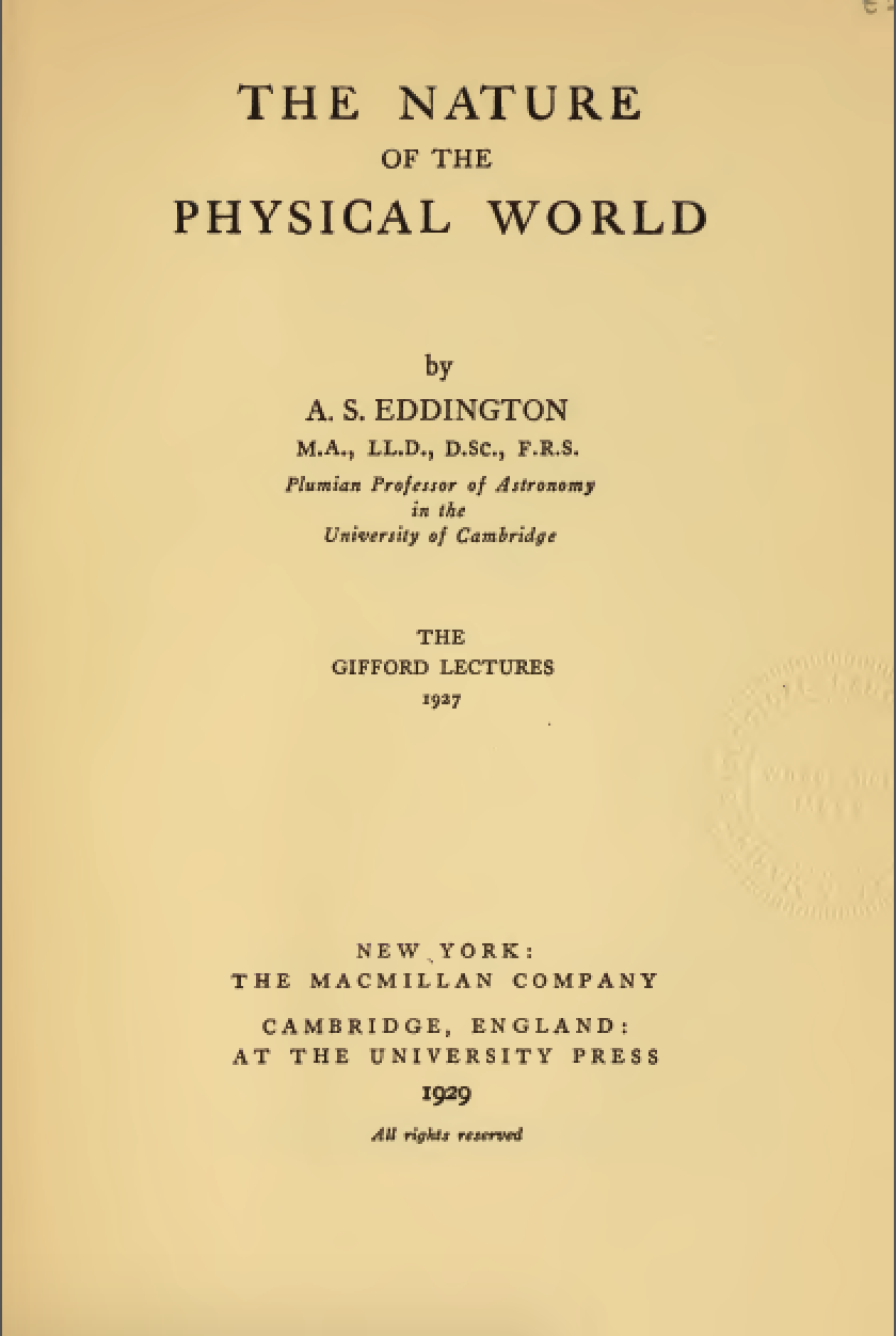
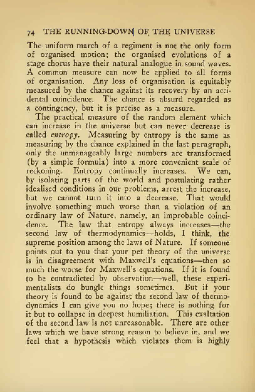
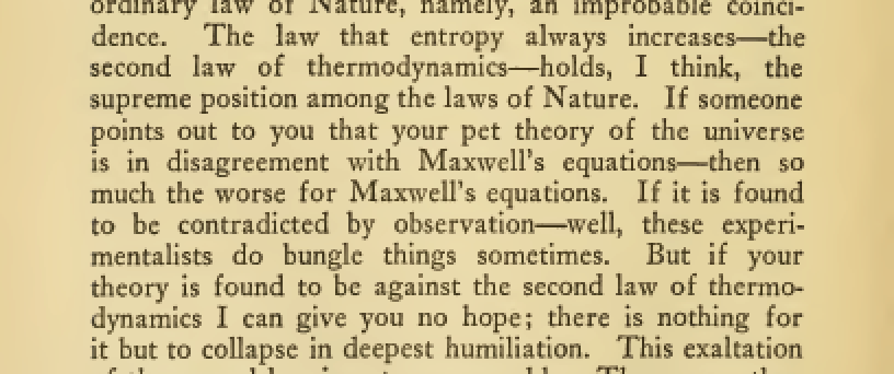
Entropy Review
Computing Expectations Example
- Consider the following distribution.
| \(y\) | 1 | 2 | 3 | 4 |
|---|---|---|---|---|
| \(P\left(y\right)\) | 0.3 | 0.2 | 0.1 | 0.4 |
- What is the mean of the distribution?
- What is the standard deviation of the distribution?
- Are the mean and standard deviation representative of the distribution form?
- What is the expected value of \(-\log P(y)\)?
Expectations Example: Answer
- We are given:
| \(y\) | 1 | 2 | 3 | 4 |
|---|---|---|---|---|
| \(P\left(y\right)\) | 0.3 | 0.2 | 0.1 | 0.4 |
| \(y^2\) | 1 | 4 | 9 | 16 |
| \(-\log(P(y))\) | 1.204 | 1.609 | 2.302 | 0.916 |
- Mean: \(1\times 0.3 + 2\times 0.2 + 3 \times 0.1 + 4 \times 0.4 = 2.6\)
- Second moment: \(1 \times 0.3 + 4 \times 0.2 + 9 \times 0.1 + 16 \times 0.4 = 8.4\)
- Variance: \(8.4 - 2.6\times 2.6 = 1.64\)
- Standard deviation: \(\sqrt{1.64} = 1.2806\)
Expectations Example: Answer II
- We are given that:
| \(y\) | 1 | 2 | 3 | 4 |
|---|---|---|---|---|
| \(P\left(y\right)\) | 0.3 | 0.2 | 0.1 | 0.4 |
| \(y^2\) | 1 | 4 | 9 | 16 |
| \(-\log(P(y))\) | 1.204 | 1.609 | 2.302 | 0.916 |
- Expectation \(-\log(P(y))\): \(0.3\times 1.204 + 0.2\times 1.609 + 0.1\times 2.302 +0.4\times 0.916 = 1.280\)
Uncertainty as a Number
Shannon entropy turns a distribution into a scalar. That number must compose across nested coarse-grainings.
- Discrete: \(H(p) = -\sum_i p_i \log p_i\) — expected surprisal
- Base 2: bits; natural log: nats
- Nested grains (this room, then the planet) must add consistently
Entropy of Common Distributions
Entropy, Distribution by Distribution
For each named family from the probability review: plot \(P\), plot \(-\log_2 P\), and form the summands \(-P\log_2 P\).
- Left: the distribution itself
- Middle: surprisal \(-\log_2 P\) (not called energy here)
- Right: \(-P\log_2 P\) — these are what sum (or integrate) to \(H\)
Bernoulli and Binomial
- Bernoulli(\(p\)): binary entropy \(-p\log_2 p-(1-p)\log_2(1-p)\)
- Binomial(\(n,p\)): no elementary closed form; same three-panel sum
- Fair coin: \(H=1\) bit
Bernoulli Entropy
Bernoulli Entropy
Bernoulli Entropy
- Fair coin \(p=\tfrac12\): \(H=1\) bit — maximal for a binary variable
- As \(p\to 0\) or \(1\): \(H\to 0\) — the outcome is nearly certain
- Closed form: \(H=-p\log_2 p-(1-p)\log_2(1-p)\)
Binomial Entropy
Binomial Entropy
Binomial Entropy
- Same visual grammar as Bernoulli: \(P\), \(-\log_2 P\), \(-P\log_2 P\)
- Surprisal is largest in the tails; weight \(P(k)\) suppresses them in \(H\)
- Large-\(n\) approximation: \(H\approx\tfrac12\log_2(2\pi e\, np(1-p))\) bits
Poisson and Multinomial
- Poisson(\(\lambda\)): numerical sum over \(k\); \(\approx\tfrac12\log_2(2\pi e\lambda)\) for large \(\lambda\)
- Categorical / one multinomial trial: \(H=-\sum_k p_k\log_2 p_k\)
- Uniform on \(K\) symbols: \(H=\log_2 K\)
Poisson Entropy
Poisson Entropy
Poisson Entropy
- Count distributions: same three-panel reading as Bernoulli / binomial
- Large-\(\lambda\) approximation: \(H\approx\tfrac12\log_2(2\pi e\lambda)\) bits
- Entropy grows only logarithmically with the rate
Multinomial / Categorical Entropy
Categorical Entropy
Categorical Entropy
- One multinomial trial \(=\) categorical: \(H=-\sum_k p_k\log_2 p_k\)
- Uniform on \(K\) symbols: \(H=\log_2 K\) — maximal
- \(n\) i.i.d. trials: entropies add; the count vector is more subtle
Gaussian
- Differential entropy \(h=-\int p\log_2 p\,\mathrm{d}y\)
- Univariate Gaussian: \(h=\tfrac12\log_2(2\pi e\sigma^2)\) bits
- Can be negative; not the same object as discrete \(H\)
Gaussian Differential Entropy
Gaussian Differential Entropy
Gaussian Differential Entropy
- Closed form: \(h=\tfrac12\log_2(2\pi e\sigma^2)\) bits
- Grows with \(\sigma\); independent of \(\mu\)
- Differential entropy \(\neq\) discrete Shannon \(H\) — can be negative
Shannon’s definition is not yet …
- … Clausius’s thermodynamic entropy (same formula, different motivation)
- … a channel-capacity theorem
Entropy: physical and anthropomorphic
- Thermodynamic \(S\) and Shannon \(H\): same form; in equilibrium \(S = k_B H\) in nats (\(S = k_B \ln 2 \cdot H\) in bits)
- \(k_B\) gives physical units (J/K); \(TS\) has units of energy
- Which degrees of freedom you count is a choice (Jaynes / Wigner: “anthropomorphic”)
- Steam tables: untampered extras (e.g. electric field) or apparent second-law violations
Joint, Conditional, Chain Rule
- \(H(X,Y)\) joint uncertainty
- \(H(X\mid Y)\) residual uncertainty after observing \(Y\)
- Chain rule: \(H(X,Y)=H(Y)+H(X\mid Y)\)
- Grouping: \(H(X)=H(G)+H(X\mid G)\) when \(G\) is a function of \(X\)
Entropy and Probability
- Probability: what things do (stochastically)
- Entropy: what things don’t do? No-go?
Prohibition
- Second law doesn’t tell you how to build an engine
- Shannon’s capacity theorem doesn’t give you a code
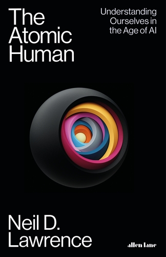
Emulate, Do Not Replicate
Anything we can measure, a machine can probably emulate. That is not the same as replicating us.
- Our intelligence is shaped by its context
- Measure a capability, fit parameters, recreate the score
- You cannot simply replicate us, because the context is specific
The Cut
If every machine capability slices something away from us, does the slicing go forever?
- Greek atomists: you stop — the world is made of what you cannot cut
- Computer scientists often say no: humans disappear
- Other answers: empathy, suffering, God
What the Machine Cannot Have
The machine cannot have our weaknesses and our vulnerabilities. They are intrinsic to us.
- Anything I can score, I can emulate
- Vulnerabilities and limitations are fundamental
- Key among them: communicate versus compute
Culture Is Compression
We built a cultural landscape so that a few bits can point at an idea you already know.
- Analogies remain a puzzle — why they work is not a derived principle
- AGI without that limitation is not general. It is specific to us
- You can emulate it, but it is not the same
What This Course Will Handle
The limitation we will treat is communication versus computation.
- Death remains the domain of theology
- Embodiment: bits we can send versus compute we can do
- You do not lose marks for believing in AGI
Information and Embodiment
Embodiment Factors
| bits/min | billions | 2,000 |
| calculations/s | ~100 billion | a billion billion |
| embodiment | 20 minutes | ~billion years |
As Delivered — Stop
We stop at embodiment. Week 3 is the heat thread, then MacKay.
- Next: Black, Carnot, Rumford, Kelvin, Joule, Clausius, Kelvin
- Then: Maxwell–Boltzmann, Gibbs, Helmholtz \(F=U-TS\)
- After that story: entropy game / MacKay / grouping
Define This Week
- How was entropy discovered? (Hydrodynamica → Maxwell / Boltzmann / Gibbs)
- \(H=-\sum_i p_i\log p_i\); no-go versus prescription (first cut)
- What are the information constraints on a human? (bandwidth, first cut)
- Continuous entropy vs relative entropy / KL (named; formalised week 3)
After This Lecture
- Next: heat thread through Helmholtz, then MacKay
- LLM probe (after \(F\)): is free energy a bound or a recipe?
Further Reading
- Chapter 1 of Lawrence (2024)
Thanks!
- company: Trent AI
- book: The Atomic Human
- twitter: @lawrennd
- The Atomic Human
- newspaper: Guardian Profile Page
- blog: http://inverseprobability.com