Week 2: Linear Algebra and Regression

[jupyter][google colab][reveal]

Neil Lawrence

Abstract:

In this session we combine the objective function perspective and the probabilistic perspective on linear regression. We motivate the importance of linear algebra by showing how much faster we can complete a linear regression using linear algebra.

Review

• Last time: Reviewed Objective Functions and gradient descent.

ML Foundations Course Notebook Setup

We install some bespoke codes for creating and saving plots as well as loading data sets.

%%capture
%pip install notutils
%pip install pods
%pip install mlai

import notutils
import pods
import mlai
import mlai.plot as plot

Learning Objectives

• Connect objective-function and probabilistic (Gaussian noise) views of linear regression.
• Derive least squares from the Gaussian likelihood and log-likelihood.
• Build and interpret simple OLS models on the Olympic data.
• Visualise optimisation landscapes (contours) and understand coordinate descent behaviour.
• Move to multivariate regression: design vectors/matrices; absorb bias into the design.
• Derive and use the direct solution (normal equations); reason about conditioning.
• Recognise numerical issues with \(\boldsymbol{ \Phi}^\top\boldsymbol{ \Phi}\) and apply QR decomposition for stable solves.
• Compare iterative optimisation (coordinate/gradient descent) with closed-form solutions and when to use each.
• Set up objective-based optimisation for multivariate linear regression.
• Be aware of related optimisation methods (Newton, quasi-Newton, momentum) and when they matter.

Lecture Timing

• Review — 5 min
• Regression examples & motivation — 5 min
• Laplace/Gauss probabilistic view — 10 min
• Univariate Gaussian & properties — 8 min
• Likelihood, log-likelihood & sum-of-squares — 12 min
• Olympic data and OLS demo — 10 min
• Coordinate ascent & contour visualisation — 10 min
• Multivariate regression & vector notation — 8 min
• Direct solution (normal equations) — 7 min
• Objective optimisation + movie body count demo — 7 min
• QR decomposition for stability — 6 min
• Wrap-up & Q&A — 2 min

Regression Examples

Regression involves predicting a real value, \(y_i\), given an input vector, \(\mathbf{ x}_i\). For example, the Tecator data involves predicting the quality of meat given spectral measurements. Or in radiocarbon dating, the C14 calibration curve maps from radiocarbon age to age measured through a back-trace of tree rings. Regression has also been used to predict the quality of board game moves given expert rated training data.

In the lecture on probability we explored how Laplace proposed that we should introduce a latent slack variable for dealing with model mismatch.

Latent Variables

Laplace’s concept was that the reason that the data doesn’t match up to the model is because of unconsidered factors, and that these might be well represented through probability densities. He tackles the challenge of the unknown factors by adding a variable, \(\epsilon\), that represents the unknown. In modern parlance we would call this a latent variable. But in the context Laplace uses it, the variable is so common that it has other names such as a “slack” variable or the noise in the system.

point 1: \(x= 1\), \(y=3\) \[ 3 = m + c + \epsilon_1 \] point 2: \(x= 3\), \(y=1\) \[ 1 = 3m + c + \epsilon_2 \] point 3: \(x= 2\), \(y=2.5\) \[ 2.5 = 2m + c + \epsilon_3 \]

Laplace’s trick has converted the overdetermined system into an underdetermined system. He has now added three variables, \(\{\epsilon_i\}_{i=1}^3\), which represent the unknown corruptions of the real world. Laplace’s idea is that we should represent that unknown corruption with a probability distribution.

A Probabilistic Process

However, it was left to an admirer of Laplace to develop a practical probability density for that purpose. It was Carl Friedrich Gauss who suggested that the Gaussian density (which at the time was unnamed!) should be used to represent this error.

The result is a noisy function, a function which has a deterministic part, and a stochastic part. This type of function is sometimes known as a probabilistic or stochastic process, to distinguish it from a deterministic process.

As we saw, Gauss used his understanding to predict where the dwarf planet Ceres could be recovered. We’ve already used the least squares algorithm to fit linear regressions. Today we’re going to motivate least squares through the probabilistic framework we introduced in Lecture 1.

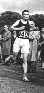
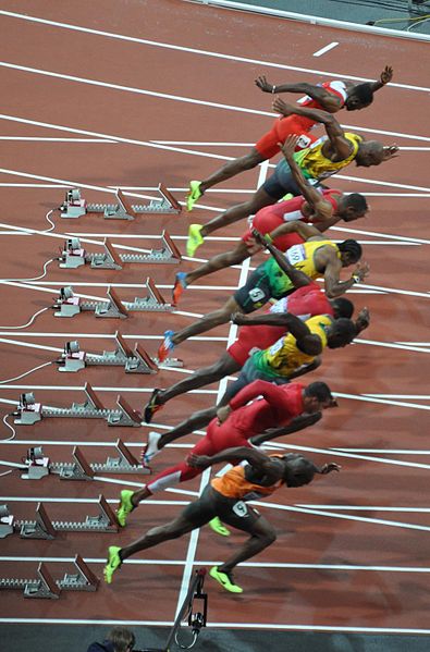
First though, we’ll introduce a data set. Since our presentation mirrors that of Rogers and Girolami, we’ll follow them in looking at Olympic sprinting data.

Olympic 100m Data

Gold medal times for Olympic 100 m runners since 1896. One of a number of Olypmic data sets collected by Rogers and Girolami (2011).

Start of the 2012 London 100m race. Image by Darren Wilkinson from Wikimedia Commons

The first thing we will do is load a standard data set for regression modelling. The data consists of the time of Olympic Gold Medal 100m winners for the Olympics from 1896 to 2012. First we load in the data and plot.

%pip install pods

import numpy as np
import pods

data = pods.datasets.olympic_100m_men()
x = data['X']
y = data['Y']

offset = y.mean()
scale = np.sqrt(y.var())

Figure: Olympic 100m wining times since 1896.

Sum of Squares Error

Last week we considered a cost function for minimization of the error. We minimised an objective that assumed used the quadratic error function, \[ E(\mathbf{ w}) = \sum_{i=1}^n \left(y_i - \mathbf{ x}_i^\top \mathbf{ w}\right)^2. \]

This week we will reinterpret the error as a probabilistic model. As Laplace suggests, we will consider the difference between our data and our model to have come from unconsidered factors which exhibit as a probability density. This leads to a more principled definition of least squares error due to Carl Friederich Gauss, but inspired by Pierre-Simon Laplace.

The Gaussian Density

The Gaussian density is perhaps the most commonly used probability density. It is defined by a mean, \(\mu\), and a variance, \(\sigma^2\). The variance is taken to be the square of the standard deviation, \(\sigma\).

\[\begin{align} p(y| \mu, \sigma^2) & = \frac{1}{\sqrt{2\pi\sigma^2}}\exp\left(-\frac{(y- \mu)^2}{2\sigma^2}\right)\\& \buildrel\triangle\over = \mathscr{N}\left(y|\mu,\sigma^2\right) \end{align}\]

Figure: The Gaussian PDF with \({\mu}=1.7\) and variance \({\sigma}^2=0.0225\). Mean shown as red line. It could represent the heights of a population of students.

Two Important Gaussian Properties

The Gaussian density has many important properties, but for the moment we’ll review two of them.

Sum of Gaussians

If we assume that a variable, \(y_i\), is sampled from a Gaussian density,

\[y_i \sim \mathscr{N}\left(\mu_i,\sigma_i^2\right)\]

Then we can show that the sum of a set of variables, each drawn independently from such a density is also distributed as Gaussian. The mean of the resulting density is the sum of the means, and the variance is the sum of the variances,

\[ \sum_{i=1}^{n} y_i \sim \mathscr{N}\left(\sum_{i=1}^n\mu_i,\sum_{i=1}^n\sigma_i^2\right) \]

Since we are very familiar with the Gaussian density and its properties, it is not immediately apparent how unusual this is. Most random variables, when you add them together, change the family of density they are drawn from. For example, the Gaussian is exceptional in this regard. Indeed, other random variables, if they are independently drawn and summed together tend to a Gaussian density. That is the central limit theorem which is a major justification for the use of a Gaussian density.

Scaling a Gaussian

Less unusual is the scaling property of a Gaussian density. If a variable, \(y\), is sampled from a Gaussian density,

\[y\sim \mathscr{N}\left(\mu,\sigma^2\right)\] and we choose to scale that variable by a deterministic value, \(w\), then the scaled variable is distributed as

\[wy\sim \mathscr{N}\left(w\mu,w^2 \sigma^2\right).\] Unlike the summing properties, where adding two or more random variables independently sampled from a family of densitites typically brings the summed variable outside that family, scaling many densities leaves the distribution of that variable in the same family of densities. Indeed, many densities include a scale parameter (e.g. the Gamma density) which is purely for this purpose. In the Gaussian the standard deviation, \(\sigma\), is the scale parameter. To see why this makes sense, let’s consider, \[z \sim \mathscr{N}\left(0,1\right),\] then if we scale by \(\sigma\) so we have, \(y=\sigma z\), we can write, \[y=\sigma z \sim \mathscr{N}\left(0,\sigma^2\right)\]

Laplace’s Idea

Laplace had the idea to augment the observations by noise, that is equivalent to considering a probability density whose mean is given by the prediction function \[p\left(y_i|x_i\right)=\frac{1}{\sqrt{2\pi\sigma^2}}\exp\left(-\frac{\left(y_i-f\left(x_i\right)\right)^{2}}{2\sigma^2}\right).\]

This is known as stochastic process. It is a function that is corrupted by noise. Laplace didn’t suggest the Gaussian density for that purpose, that was an innovation from Carl Friederich Gauss, which is what gives the Gaussian density its name.

Height as a Function of Weight

In the standard Gaussian, parameterized by mean and variance, make the mean a linear function of an input.

This leads to a regression model. \[ \begin{align*} y_i=&f\left(x_i\right)+\epsilon_i,\\ \epsilon_i \sim & \mathscr{N}\left(0,\sigma^2\right). \end{align*} \]

Assume \(y_i\) is height and \(x_i\) is weight.

Sum of Squares Error

Legendre

Minimising the sum of squares error was first proposed by Legendre in 1805 (Legendre, 1805). His book, which was on the orbit of comets, is available on Google books, we can take a look at the relevant page by calling the code below.

Figure: Legendre’s book was on the determination of orbits of comets. This page describes the formulation of least squares

Of course, the main text is in French, but the key part we are interested in can be roughly translated as

In most matters where we take measures data through observation, the most accurate results they can offer, it is almost always leads to a system of equations of the form \[E = a + bx + cy + fz + etc .\] where \(a\), \(b\), \(c\), \(f\) etc are the known coefficients and \(x\), \(y\), \(z\) etc are unknown and must be determined by the condition that the value of E is reduced, for each equation, to an amount or zero or very small.

He continues

Of all the principles that we can offer for this item, I think it is not broader, more accurate, nor easier than the one we have used in previous research application, and that is to make the minimum sum of the squares of the errors. By this means, it is between the errors a kind of balance that prevents extreme to prevail, is very specific to make known the state of the closest to the truth system. The sum of the squares of the errors \(E^2 + \left.E^\prime\right.^2 + \left.E^{\prime\prime}\right.^2 + etc\) being \[\begin{align*} &(a + bx + cy + fz + etc)^2 \\ + &(a^\prime + b^\prime x + c^\prime y + f^\prime z + etc ) ^2\\ + &(a^{\prime\prime} + b^{\prime\prime}x + c^{\prime\prime}y + f^{\prime\prime}z + etc )^2 \\ + & etc \end{align*}\] if we wanted a minimum, by varying x alone, we will have the equation …

This is the earliest know printed version of the problem of least squares. The notation, however, is a little awkward for mordern eyes. In particular Legendre doesn’t make use of the sum sign, \[ \sum_{i=1}^3 z_i = z_1 + z_2 + z_3 \] nor does he make use of the inner product.

In our notation, if we were to do linear regression, we would need to subsititue: \[\begin{align*} a &\leftarrow y_1-c, \\ a^\prime &\leftarrow y_2-c,\\ a^{\prime\prime} &\leftarrow y_3 -c,\\ \text{etc.} \end{align*}\] to introduce the data observations \(\{y_i\}_{i=1}^{n}\) alongside \(c\), the offset. We would then introduce the input locations \[\begin{align*} b & \leftarrow x_1,\\ b^\prime & \leftarrow x_2,\\ b^{\prime\prime} & \leftarrow x_3\\ \text{etc.} \end{align*}\] and finally the gradient of the function \[x \leftarrow -m.\] The remaining coefficients (\(c\) and \(f\)) would then be zero. That would give us \[\begin{align*} &(y_1 - (mx_1+c))^2 \\ + &(y_2 -(mx_2 + c))^2\\ + &(y_3 -(mx_3 + c))^2 \\ + & \text{etc.} \end{align*}\] which we would write in the modern notation for sums as \[ \sum_{i=1}^n(y_i-(mx_i + c))^2 \] which is recognised as the sum of squares error for a linear regression.

This shows the advantage of modern summation operator, \(\sum\), in keeping our mathematical notation compact. Whilst it may look more complicated the first time you see it, understanding the mathematical rules that go around it, allows us to go much further with the notation.

Inner products (or dot products) are similar. They allow us to write \[ \sum_{i=1}^q u_i v_i \] in vector notation, \(\mathbf{u}^\top\mathbf{v}.\)

Here we are using bold face to represent vectors, and we assume that the individual elements of a vector \(\mathbf{z}\) are given as a series of scalars \[ \mathbf{z} = \begin{bmatrix} z_1\\ z_2\\ \vdots\\ z_n \end{bmatrix} \] which are each indexed by their position in the vector.

Unfortunately for Legendre, Gauss had already used the least squares method in his recoveroy of Ceres. This led to a priority dispute which Gauss’s unpublished use being established as predating Legendre’s.

Olympic Marathon Data

Gold medal times for Olympic Marathon since 1896. Marathons before 1924 didn’t have a standardized distance. Present results using pace per km. In 1904 Marathon was badly organized leading to very slow times.

Image from Wikimedia Commons

The Olympic Marathon data is a standard dataset for regression modelling. The data consists of the pace of Olympic Gold Medal Marathon winners for the Olympics from 1896 to present. Let’s load in the data and plot.

import numpy as np
import pods

data = pods.datasets.olympic_marathon_men()
x = data['X']
y = data['Y']

offset = y.mean()
scale = np.sqrt(y.var())
yhat = (y - offset)/scale

Figure: Olympic marathon pace times since 1896.

Things to notice about the data include the outlier in 1904, in that year the Olympics was in St Louis, USA. Organizational problems and challenges with dust kicked up by the cars following the race meant that participants got lost, and only very few participants completed. More recent years see more consistently quick marathons.

Alan Turing

Figure: Alan Turing, in 1946 he was only 11 minutes slower than the winner of the 1948 games. Would he have won a hypothetical games held in 1946? Source: Alan Turing Internet Scrapbook.

If we had to summarise the objectives of machine learning in one word, a very good candidate for that word would be generalization. What is generalization? From a human perspective it might be summarised as the ability to take lessons learned in one domain and apply them to another domain. If we accept the definition given in the first session for machine learning, \[ \text{data} + \text{model} \stackrel{\text{compute}}{\rightarrow} \text{prediction} \] then we see that without a model we can’t generalise: we only have data. Data is fine for answering very specific questions, like “Who won the Olympic Marathon in 2012?” because we have that answer stored, however, we are not given the answer to many other questions. For example, Alan Turing was a formidable marathon runner, in 1946 he ran a time 2 hours 46 minutes (just under four minutes per kilometer, faster than I and most of the other Endcliffe Park Run runners can do 5 km). What is the probability he would have won an Olympics if one had been held in 1946?

To answer this question we need to generalize, but before we formalize the concept of generalization let’s introduce some formal representation of what it means to generalize in machine learning.

Running Example: Olympic Marathons

Note that x and y are not pandas data frames for this example, they are just arrays of dimensionality \(n\times 1\), where \(n\) is the number of data.

The aim of this lab is to have you coding linear regression in python. We will do it in two ways, once using iterative updates (coordinate ascent) and then using linear algebra. The linear algebra approach will not only work much better, it is also easy to extend to multiple input linear regression and non-linear regression using basis functions.

Maximum Likelihood: Iterative Solution

Now we will take the maximum likelihood approach we derived in the lecture to fit a line, \(y_i=mx_i + c\), to the data you’ve plotted. We are trying to minimize the error function, \[ E(m, c) = \sum_{i=1}^n(y_i-mx_i-c)^2, \] with respect to \(m\), \(c\) and \(\sigma^2\). We can start with an initial guess for \(m\),

m = -0.4
c = 80

Then we use the maximum likelihood update to find an estimate for the offset, \(c\).

Coordinate Descent

In the movie recommender system example, we minimised the objective function by steepest descent based gradient methods. Our updates required us to compute the gradient at the position we were located, then to update the gradient according to the direction of steepest descent. This time, we will take another approach. It is known as coordinate descent. In coordinate descent, we choose to move one parameter at a time. Ideally, we design an algorithm that at each step moves the parameter to its minimum value. At each step we choose to move the individual parameter to its minimum.

To find the minimum, we look for the point in the curve where the gradient is zero. This can be found by taking the gradient of \(E(m,c)\) with respect to the parameter.

Update for Offset

Let’s consider the parameter \(c\) first. The gradient goes nicely through the summation operator, and we obtain \[ \frac{\text{d}E(m,c)}{\text{d}c} = -\sum_{i=1}^n2(y_i-mx_i-c). \] Now we want the point that is a minimum. A minimum is an example of a stationary point, the stationary points are those points of the function where the gradient is zero. They are found by solving the equation for \(\frac{\text{d}E(m,c)}{\text{d}c} = 0\). Substituting in to our gradient, we can obtain the following equation, \[ 0 = -\sum_{i=1}^n2(y_i-mx_i-c) \] which can be reorganised as follows, \[ c^* = \frac{\sum_{i=1}^n(y_i-m^*x_i)}{n}. \] The fact that the stationary point is easily extracted in this manner implies that the solution is unique. There is only one stationary point for this system. Traditionally when trying to determine the type of stationary point we have encountered we now compute the second derivative, \[ \frac{\text{d}^2E(m,c)}{\text{d}c^2} = 2n. \] The second derivative is positive, which implies that we have found a minimum of the function. This means that setting \(c\) using this update will take us to the lowest point along that axes.

# set c to the minimum
c = (y - m*x).mean()
print(c)

Update for Slope

Now we have the offset set to the minimum value, in coordinate descent, the next step is to optimise another parameter. Only one further parameter remains. That is the slope of the system.

Now we can turn our attention to the slope. We once again peform the same set of computations to find the minima. We end up with an update equation of the following form.

\[m^* = \frac{\sum_{i=1}^n(y_i - c)x_i}{\sum_{i=1}^nx_i^2}\]

Communication of mathematics in data science is an essential skill, in a moment, you will be asked to rederive the equation above. Before we do that, however, we will briefly review how to write mathematics in the notebook.

\(\LaTeX\) for Maths

These cells use Markdown format. You can include maths in your markdown using \(\LaTeX\) syntax, all you have to do is write your answer inside dollar signs, as follows:

To write a fraction, we write $\frac{a}{b}$, and it will display like this \(\frac{a}{b}\). To write a subscript we write $a_b$ which will appear as \(a_b\). To write a superscript (for example in a polynomial) we write $a^b$ which will appear as \(a^b\). There are lots of other macros as well, for example we can do greek letters such as $\alpha, \beta, \gamma$ rendering as \(\alpha, \beta, \gamma\). And we can do sum and intergral signs as $\sum \int \int$.

You can combine many of these operations together for composing expressions.

Exercise 1

Convert the following python code expressions into \(\LaTeX\)j, writing your answers below. In each case write your answer as a single equality (i.e. your maths should only contain one expression, not several lines of expressions). For the purposes of your \(\LaTeX\) please assume that x and w are \(n\) dimensional vectors.

(a) f = x.sum()

(b) m = x.mean()

(c) g = (x*w).sum()

Fixed Point Updates

\[ \begin{aligned} c^{*}=&\frac{\sum _{i=1}^{n}\left(y_i-m^{*}x_i\right)}{n},\\ m^{*}=&\frac{\sum _{i=1}^{n}x_i\left(y_i-c^{*}\right)}{\sum _{i=1}^{n}x_i^{2}},\\ \left.\sigma^2\right.^{*}=&\frac{\sum _{i=1}^{n}\left(y_i-m^{*}x_i-c^{*}\right)^{2}}{n} \end{aligned} \]

Gradient With Respect to the Slope

Now that you’ve had a little training in writing maths with \(\LaTeX\), we will be able to use it to answer questions. The next thing we are going to do is a little differentiation practice.

Exercise 2

Derive the the gradient of the objective function with respect to the slope, \(m\). Rearrange it to show that the update equation written above does find the stationary points of the objective function. By computing its derivative show that it’s a minimum.

m = ((y - c)*x).sum()/(x**2).sum()
print(m)

We can have a look at how good our fit is by computing the prediction across the input space. First create a vector of ‘test points,’

import numpy as np

x_test = np.linspace(1890, 2020, 130)[:, None]

Now use this vector to compute some test predictions,

f_test = m*x_test + c

Now plot those test predictions with a blue line on the same plot as the data,

import matplotlib.pyplot as plt

plt.plot(x_test, f_test, 'b-')
plt.plot(x, y, 'rx')

The fit isn’t very good, we need to iterate between these parameter updates in a loop to improve the fit, we have to do this several times,

for i in np.arange(10):
    m = ((y - c)*x).sum()/(x*x).sum()
    c = (y-m*x).sum()/y.shape[0]
print(m)
print(c)

And let’s try plotting the result again

f_test = m*x_test + c
plt.plot(x_test, f_test, 'b-')
plt.plot(x, y, 'rx')

Clearly we need more iterations than 10! In the next question you will add more iterations and report on the error as optimisation proceeds.

Coordiate Descent Algorithm

Let’s run the complete coordiante descent algorithm and visualise how the parameters evolve over multiple iterations. The animation will show the path taken through parameter space as the algorithm navigates toward the minimum of the error surface.

Exercise 3

There is a problem here, we seem to need many interations to get to a good solution. Let’s explore what’s going on. Write code which alternates between updates of c and m. Include the following features in your code.

1. Initialise with m=-0.4 and c=80.
2. Every 10 iterations compute the value of the objective function for the training data and print it to the screen.
3. Cause the code to stop running when the error changes over less than 10 iterations is smaller than \(1\times 10^{-4}\). This is known as a stopping criterion.

Why do we need so many iterations to get to the solution?

Let’s recreate our data set we used for the iterative fitting so we can visualise the optimisation process.

m_true  = 1.4
c_true = -3.1
np.random.seed(42)
x = np.random.normal(size=(4, 1))
noise = np.random.normal(scale=0.5, size=(4, 1)) # standard deviation of the noise is 0.5
y = m_true*x + c_true + noise

Contour Plot of Error Function

To understand how the least squares algorithm works, it’s helpful to visualize the error function as a surface in parameter space. Since we have two parameters (\(m\) and \(c\)), our error function \(E(m, c)\) defines a surface in 3D space where the height at any point represents the error for that combination of parameters.

The global minimum of this surface is given by the optimal parameter values that best fit our data according to the least squares objective. By visualising this surface through contour plots, we can gain intuition about the optimization landscape and understand why gradient-based methods work effectively for this problem.

First, we create vectors of parameter values to explore around the true values we used to generate the data. We sample points in a range around the true parameters to see how the error function behaves in the local neighborhood.

# create an array of linearly separated values around m_true
m_vals = np.linspace(m_true-3, m_true+3, 100) 
# create an array of linearly separated values around c_true
c_vals = np.linspace(c_true-3, c_true+3, 100)

Next, we create a 2D grid from these parameter vectors. This grid allows us to evaluate the error function at every combination of \(m\) and \(c\) values, giving us a complete picture of the error surface over the parameter space we’re exploring.

m_grid, c_grid = np.meshgrid(m_vals, c_vals)

Now we compute the error function at each combination of parameters. For each point in our grid, we:

1. Use the parameter values to make predictions: \(\hat{y}_i = m \cdot x_i + c\)
   
2. Calculate the squared errors: \((y_i - \hat{y}_i)^2\)
3. Sum these squared errors to get the total error for that parameter combination

This gives us the complete error surface that we can then visualize. The nested loop structure evaluates the sum of squared errors formula at each \((m, c)\) coordinate in our grid.

E_grid = np.zeros((100, 100))
for i in range(100):
    for j in range(100):
        E_grid[i, j] = ((y - m_grid[i, j]*x - c_grid[i, j])**2).sum()

With our error surface computed, we can now create a contour plot to visualize the optimization landscape. A contour plot shows lines of equal error value, similar to elevation contours on a topographic map.

Insights from this visualisation include:

• Bowl-shaped surface: For linear regression with least squares, the error surface is a smooth, convex bowl with a unique global minimum
• Contour lines: Each contour represents parameter combinations that yield the same error value
• Minimum location: The centre of the concentric ellipses shows where the error is minimized - this should be close to our true parameter values

This visualisation helps explain why least squares regression has nice mathematical properties and why optimisation algorithms converge reliably to the solution.

Figure: Contours of the objective function for linear regression by minimizing least squares.

The contour plot reveals the characteristic elliptical shape of the least squares error surface. The concentric ellipses represent increasing levels of error as we move away from the optimal parameters.

Key observations from this visualization:

• Convex optimisation: The smooth, bowl-shaped surface guarantees that any local minimum is also the global minimum
• Parameter sensitivity: The shape of the ellipses tells us how sensitive the error is to changes in each parameter
• Optimization efficiency: The regular, predictable shape means we can develop optimisation methods that will converge quickly and reliably
• True parameter location: The minimum should occur very close to our known true values (\(m_{true} = 1.4\), \(c_{true} = -3.1\))

Warning: This visualisation is great for giving some intuition, but can be quite misleading about how these objective funcitons look in very high dimensions. Unfortunately high dimensions are much harder to visualise.

Regression Coordiate Fit

Now we’ll run Each frame shows:

• Current position: The green star indicating our current parameter estimates
• Error contours: The background showing the error landscape
• Path: The trajectory we’ve taken from the starting point to the current position

Watch how the algorithm follows a “staircase” path that converges towards the minimum. Note that the more correlated \(m\) and \(c\) are (principle axes of the ellipse contours is diagonal) the slower the convergence towards the minimum demonstrating the potential limitation of coordinate descent.

Figure: Coordinate descent for linear regression showing the path after 20 updates between \(c\) and \(m\).

Exercise 4

Why does the coordiate descent converge so quickly for the toy data example, but take so long for the Marathon data?

Important Concepts Not Covered

• Other optimization methods:
  • Second order methods, conjugate gradient, quasi-Newton and Newton.
• Effective heuristics such as momentum.
• Local vs global solutions.

Multivariate Regression

What if we’re faced with a multivariate regression. For example, we might try and predict height given weight and gender.

Log Likelihood for Multivariate Regression

Quadratic Loss

Now we’ve identified the empirical risk with the loss, we’ll use \(E(\mathbf{ w})\) to represent our objective function. \[ E(\mathbf{ w}) = \sum_{i=1}^n\left(y_i - f(\mathbf{ x}_i, \mathbf{ w})\right)^2 \] gives us our objective.

In the case of the linear prediction function, we can substitute \(f(\mathbf{ x}_i, \mathbf{ w}) = \mathbf{ w}^\top \mathbf{ x}_i\). \[ E(\mathbf{ w}) = \sum_{i=1}^n\left(y_i - \mathbf{ w}^\top \mathbf{ x}_i\right)^2 \] To compute the gradient of the objective, we first expand the brackets.

Bracket Expansion

\[ \begin{align*} E(\mathbf{ w},\sigma^2) = & \frac{n}{2}\log \sigma^2 + \frac{1}{2\sigma^2}\sum _{i=1}^{n}y_i^{2}-\frac{1}{\sigma^2}\sum _{i=1}^{n}y_i\mathbf{ w}^{\top}\mathbf{ x}_i\\&+\frac{1}{2\sigma^2}\sum _{i=1}^{n}\mathbf{ w}^{\top}\mathbf{ x}_i\mathbf{ x}_i^{\top}\mathbf{ w} +\text{const}.\\ = & \frac{n}{2}\log \sigma^2 + \frac{1}{2\sigma^2}\sum _{i=1}^{n}y_i^{2}-\frac{1}{\sigma^2} \mathbf{ w}^\top\sum_{i=1}^{n}\mathbf{ x}_iy_i\\&+\frac{1}{2\sigma^2} \mathbf{ w}^{\top}\left[\sum _{i=1}^{n}\mathbf{ x}_i\mathbf{ x}_i^{\top}\right]\mathbf{ w}+\text{const}. \end{align*} \]

Solution with Linear Algebra

In this section we’re going compute the minimum of the quadratic loss with respect to the parameters. When we do this, we’ll also review linear algebra. We will represent all our errors and functions in the form of matrices and vectors.

Linear algebra is just a shorthand for performing lots of multiplications and additions simultaneously. What does it have to do with our system then? Well, the first thing to note is that the classic linear function we fit for a one-dimensional regression has the form: \[ f(x) = mx + c \] the classical form for a straight line. From a linear algebraic perspective, we are looking for multiplications and additions. We are also looking to separate our parameters from our data. The data is the givens. In French the word is données literally translated means givens that’s great, because we don’t need to change the data, what we need to change are the parameters (or variables) of the model. In this function the data comes in through \(x\), and the parameters are \(m\) and \(c\).

What we’d like to create is a vector of parameters and a vector of data. Then we could represent the system with vectors that represent the data, and vectors that represent the parameters.

We look to turn the multiplications and additions into a linear algebraic form, we have one multiplication (\(m\times c\)) and one addition (\(mx + c\)). But we can turn this into an inner product by writing it in the following way, \[ f(x) = m \times x + c \times 1, \] in other words, we’ve extracted the unit value from the offset, \(c\). We can think of this unit value like an extra item of data, because it is always given to us, and it is always set to 1 (unlike regular data, which is likely to vary!). We can therefore write each input data location, \(\mathbf{ x}\), as a vector \[ \mathbf{ x}= \begin{bmatrix} 1\\ x\end{bmatrix}. \]

Now we choose to also turn our parameters into a vector. The parameter vector will be defined to contain \[ \mathbf{ w}= \begin{bmatrix} c \\ m\end{bmatrix} \] because if we now take the inner product between these two vectors we recover \[ \mathbf{ x}\cdot\mathbf{ w}= 1 \times c + x \times m = mx + c \] In numpy we can define this vector as follows

import numpy as np

# define the vector w
w = np.zeros(shape=(2, 1))
w[0] = m
w[1] = c

This gives us the equivalence between original operation and an operation in vector space. Whilst the notation here isn’t a lot shorter, the beauty is that we will be able to add as many features as we like and keep the same representation. In general, we are now moving to a system where each of our predictions is given by an inner product. When we want to represent a linear product in linear algebra, we tend to do it with the transpose operation, so since we have \(\mathbf{a}\cdot\mathbf{b} = \mathbf{a}^\top\mathbf{b}\) we can write \[ f(\mathbf{ x}_i) = \mathbf{ x}_i^\top\mathbf{ w}. \] Where we’ve assumed that each data point, \(\mathbf{ x}_i\), is now written by appending a 1 onto the original vector \[ \mathbf{ x}_i = \begin{bmatrix} 1 \\ x_i \end{bmatrix} \]

Design Matrix

We can do this for the entire data set to form a design matrix \(\mathbf{X}\), \[ \mathbf{X} = \begin{bmatrix} \mathbf{ x}_1^\top \\\ \mathbf{ x}_2^\top \\\ \vdots \\\ \mathbf{ x}_n^\top \end{bmatrix} = \begin{bmatrix} 1 & x_1 \\\ 1 & x_2 \\\ \vdots & \vdots \\\ 1 & x_n \end{bmatrix}, \] which in numpy can be done with the following commands:

import numpy as np

X = np.hstack((np.ones_like(x), x))
print(X)

Writing the Objective with Linear Algebra

When we think of the objective function, we can think of it as the errors where the error is defined in a similar way to what it was in Legendre’s day \(y_i - f(\mathbf{ x}_i)\), in statistics these errors are also sometimes called residuals. So, we can think as the objective and the prediction function as two separate parts, first we have, \[ E(\mathbf{ w}) = \sum_{i=1}^n(y_i - f(\mathbf{ x}_i; \mathbf{ w}))^2, \] where we’ve made the function \(f(\cdot)\)’s dependence on the parameters \(\mathbf{ w}\) explicit in this equation. Then we have the definition of the function itself, \[ f(\mathbf{ x}_i; \mathbf{ w}) = \mathbf{ x}_i^\top \mathbf{ w}. \] Let’s look again at these two equations and see if we can identify any inner products. The first equation is a sum of squares, which is promising. Any sum of squares can be represented by an inner product, \[ a = \sum_{i=1}^{k} b^2_i = \mathbf{b}^\top\mathbf{b}. \] If we wish to represent \(E(\mathbf{ w})\) in this way, all we need to do is convert the sum operator to an inner product. We can get a vector from that sum operator by placing both \(y_i\) and \(f(\mathbf{ x}_i; \mathbf{ w})\) into vectors, which we do by defining \[ \mathbf{ y}= \begin{bmatrix}y_1\\ y_2\\ \vdots \\ y_n\end{bmatrix} \] and defining \[ \mathbf{ f}(\mathbf{ x}_1; \mathbf{ w}) = \begin{bmatrix}f(\mathbf{ x}_1; \mathbf{ w})\\ f(\mathbf{ x}_2; \mathbf{ w})\\ \vdots \\ f(\mathbf{ x}_n; \mathbf{ w})\end{bmatrix}. \] The second of these is a vector-valued function. This term may appear intimidating, but the idea is straightforward. A vector valued function is simply a vector whose elements are themselves defined as functions, i.e., it is a vector of functions, rather than a vector of scalars. The idea is so straightforward, that we are going to ignore it for the moment, and barely use it in the derivation. But it will reappear later when we introduce basis functions. So, we will for the moment ignore the dependence of \(\mathbf{ f}\) on \(\mathbf{ w}\) and \(\mathbf{X}\) and simply summarise it by a vector of numbers \[ \mathbf{ f}= \begin{bmatrix}f_1\\f_2\\ \vdots \\ f_n\end{bmatrix}. \] This allows us to write our objective in the folowing, linear algebraic form, \[ E(\mathbf{ w}) = (\mathbf{ y}- \mathbf{ f})^\top(\mathbf{ y}- \mathbf{ f}) \] from the rules of inner products. But what of our matrix \(\mathbf{X}\) of input data? At this point, we need to dust off matrix-vector multiplication. Matrix multiplication is simply a convenient way of performing many inner products together, and it’s exactly what we need to summarize the operation \[ f_i = \mathbf{ x}_i^\top\mathbf{ w}. \] This operation tells us that each element of the vector \(\mathbf{ f}\) (our vector valued function) is given by an inner product between \(\mathbf{ x}_i\) and \(\mathbf{ w}\). In other words, it is a series of inner products. Let’s look at the definition of matrix multiplication, it takes the form \[ \mathbf{c} = \mathbf{B}\mathbf{a}, \] where \(\mathbf{c}\) might be a \(k\) dimensional vector (which we can interpret as a \(k\times 1\) dimensional matrix), and \(\mathbf{B}\) is a \(k\times k\) dimensional matrix and \(\mathbf{a}\) is a \(k\) dimensional vector (\(k\times 1\) dimensional matrix).

The result of this multiplication is of the form \[ \begin{bmatrix}c_1\\c_2 \\ \vdots \\ a_k\end{bmatrix} = \begin{bmatrix} b_{1,1} & b_{1, 2} & \dots & b_{1, k} \\ b_{2, 1} & b_{2, 2} & \dots & b_{2, k} \\ \vdots & \vdots & \ddots & \vdots \\ b_{k, 1} & b_{k, 2} & \dots & b_{k, k} \end{bmatrix} \begin{bmatrix}a_1\\a_2 \\ \vdots\\ c_k\end{bmatrix} = \begin{bmatrix} b_{1, 1}a_1 + b_{1, 2}a_2 + \dots + b_{1, k}a_k\\ b_{2, 1}a_1 + b_{2, 2}a_2 + \dots + b_{2, k}a_k \\ \vdots\\ b_{k, 1}a_1 + b_{k, 2}a_2 + \dots + b_{k, k}a_k\end{bmatrix}. \] We see that each element of the result, \(\mathbf{a}\) is simply the inner product between each row of \(\mathbf{B}\) and the vector \(\mathbf{c}\). Because we have defined each element of \(\mathbf{ f}\) to be given by the inner product between each row of the design matrix and the vector \(\mathbf{ w}\) we now can write the full operation in one matrix multiplication,

\[ \mathbf{ f}= \mathbf{X}\mathbf{ w}. \]

import numpy as np

f = X@w # The @ sign performs matrix multiplication

Combining this result with our objective function, \[ E(\mathbf{ w}) = (\mathbf{ y}- \mathbf{ f})^\top(\mathbf{ y}- \mathbf{ f}) \] we find we have defined the model with two equations. One equation tells us the form of our predictive function and how it depends on its parameters, the other tells us the form of our objective function.

resid = (y-f)
E = np.dot(resid.T, resid) # matrix multiplication on a single vector is equivalent to a dot product.
print("Error function is:", E)

Objective Optimization

Our model has now been defined with two equations: the prediction function and the objective function. Now we will use multivariate calculus to define an algorithm to fit the model. The separation between model and algorithm is important and is often overlooked. Our model contains a function that shows how it will be used for prediction, and a function that describes the objective function we need to optimize to obtain a good set of parameters.

The model linear regression model we have described is still the same as the one we fitted above with a coordinate ascent algorithm. We have only played with the notation to obtain the same model in a matrix and vector notation. However, we will now fit this model with a different algorithm, one that is much faster. It is such a widely used algorithm that from the end user’s perspective it doesn’t even look like an algorithm, it just appears to be a single operation (or function). However, underneath the computer calls an algorithm to find the solution. Further, the algorithm we obtain is very widely used, and because of this it turns out to be highly optimized.

Once again, we are going to try and find the stationary points of our objective by finding the stationary points. However, the stationary points of a multivariate function, are a little bit more complex to find. As before we need to find the point at which the gradient is zero, but now we need to use multivariate calculus to find it. This involves learning a few additional rules of differentiation (that allow you to do the derivatives of a function with respect to vector), but in the end it makes things quite a bit easier. We define vectorial derivatives as follows, \[ \frac{\text{d}E(\mathbf{ w})}{\text{d}\mathbf{ w}} = \begin{bmatrix}\frac{\text{d}E(\mathbf{ w})}{\text{d}w_1}\\\frac{\text{d}E(\mathbf{ w})}{\text{d}w_2}\end{bmatrix}. \] where \(\frac{\text{d}E(\mathbf{ w})}{\text{d}w_1}\) is the partial derivative of the error function with respect to \(w_1\).

Differentiation through multiplications and additions is relatively straightforward, and since linear algebra is just multiplication and addition, then its rules of differentiation are quite straightforward too, but slightly more complex than regular derivatives.

Multivariate Derivatives

We will need two rules of multivariate or matrix differentiation. The first is differentiation of an inner product. By remembering that the inner product is made up of multiplication and addition, we can hope that its derivative is quite straightforward, and so it proves to be. We can start by thinking about the definition of the inner product, \[ \mathbf{a}^\top\mathbf{z} = \sum_{i} a_i z_i, \] which if we were to take the derivative with respect to \(z_k\) would simply return the gradient of the one term in the sum for which the derivative was non-zero, that of \(a_k\), so we know that \[ \frac{\text{d}}{\text{d}z_k} \mathbf{a}^\top \mathbf{z} = a_k \] and by our definition for multivariate derivatives, we can simply stack all the partial derivatives of this form in a vector to obtain the result that \[ \frac{\text{d}}{\text{d}\mathbf{z}} \mathbf{a}^\top \mathbf{z} = \mathbf{a}. \] The second rule that’s required is differentiation of a ‘matrix quadratic.’ A scalar quadratic in \(z\) with coefficient \(c\) has the form \(cz^2\). If \(\mathbf{z}\) is a \(k\times 1\) vector and \(\mathbf{C}\) is a \(k \times k\) matrix of coefficients then the matrix quadratic form is written as \(\mathbf{z}^\top \mathbf{C}\mathbf{z}\), which is itself a scalar quantity, but it is a function of a vector.

Matching Dimensions in Matrix Multiplications

There’s a trick for telling a multiplication leads to a scalar result. When you are doing mathematics with matrices, it’s always worth pausing to perform a quick sanity check on the dimensions. Matrix multplication only works when the dimensions match. To be precise, the ‘inner’ dimension of the matrix must match. What is the inner dimension? If we multiply two matrices \(\mathbf{A}\) and \(\mathbf{B}\), the first of which has \(k\) rows and \(\ell\) columns and the second of which has \(p\) rows and \(q\) columns, then we can check whether the multiplication works by writing the dimensionalities next to each other, \[ \mathbf{A} \mathbf{B} \rightarrow (k \times \underbrace{\ell)(p}_\text{inner dimensions} \times q) \rightarrow (k\times q). \] The inner dimensions are the two inside dimensions, \(\ell\) and \(p\). The multiplication will only work if \(\ell=p\). The result of the multiplication will then be a \(k\times q\) matrix: this dimensionality comes from the ‘outer dimensions.’ Note that matrix multiplication is not commutative. And if you change the order of the multiplication, \[ \mathbf{B} \mathbf{A} \rightarrow (\ell \times \underbrace{k)(q}_\text{inner dimensions} \times p) \rightarrow (\ell \times p). \] Firstly, it may no longer even work, because now the condition is that \(k=q\), and secondly the result could be of a different dimensionality. An exception is if the matrices are square matrices (e.g., same number of rows as columns) and they are both symmetric. A symmetric matrix is one for which \(\mathbf{A}=\mathbf{A}^\top\), or equivalently, \(a_{i,j} = a_{j,i}\) for all \(i\) and \(j\).

For applying and developing machine learning algorithms you should get familiar with working with matrices and vectors. You should have come across them before, but you may not have used them as extensively as we are doing now. It’s worth getting used to using this trick to check your work and ensure you know what the dimension of an output matrix should be. For our matrix quadratic form, it turns out that we can see it as a special type of inner product. \[ \mathbf{z}^\top\mathbf{C}\mathbf{z} \rightarrow (1\times \underbrace{k) (k}_\text{inner dimensions}\times k) (k\times 1) \rightarrow \mathbf{b}^\top\mathbf{z} \] where \(\mathbf{b} = \mathbf{C}\mathbf{z}\) so therefore the result is a scalar, \[ \mathbf{b}^\top\mathbf{z} \rightarrow (1\times \underbrace{k) (k}_\text{inner dimensions}\times 1) \rightarrow (1\times 1) \] where a \((1\times 1)\) matrix is recognised as a scalar.

This implies that we should be able to differentiate this form, and indeed the rule for its differentiation is slightly more complex than the inner product, but still quite simple, \[ \frac{\text{d}}{\text{d}\mathbf{z}} \mathbf{z}^\top\mathbf{C}\mathbf{z}= \mathbf{C}\mathbf{z} + \mathbf{C}^\top \mathbf{z}. \] Note that in the special case where \(\mathbf{C}\) is symmetric then we have \(\mathbf{C} = \mathbf{C}^\top\) and the derivative simplifies to \[ \frac{\text{d}}{\text{d}\mathbf{z}} \mathbf{z}^\top\mathbf{C}\mathbf{z}= 2\mathbf{C}\mathbf{z}. \]

Differentiate the Objective

First, we need to compute the full objective by substituting our prediction function into the objective function to obtain the objective in terms of \(\mathbf{ w}\). Doing this we obtain \[ E(\mathbf{ w})= (\mathbf{ y}- \mathbf{X}\mathbf{ w})^\top (\mathbf{ y}- \mathbf{X}\mathbf{ w}). \] We now need to differentiate this quadratic form to find the minimum. We differentiate with respect to the vector \(\mathbf{ w}\). But before we do that, we’ll expand the brackets in the quadratic form to obtain a series of scalar terms. The rules for bracket expansion across the vectors are similar to those for the scalar system giving, \[ (\mathbf{a} - \mathbf{b})^\top (\mathbf{c} - \mathbf{d}) = \mathbf{a}^\top \mathbf{c} - \mathbf{a}^\top \mathbf{d} - \mathbf{b}^\top \mathbf{c} + \mathbf{b}^\top \mathbf{d} \] which substituting for \(\mathbf{a} = \mathbf{c} = \mathbf{ y}\) and \(\mathbf{b}=\mathbf{d} = \mathbf{X}\mathbf{ w}\) gives \[ E(\mathbf{ w})= \mathbf{ y}^\top\mathbf{ y}- 2\mathbf{ y}^\top\mathbf{X}\mathbf{ w}+ \mathbf{ w}^\top\mathbf{X}^\top\mathbf{X}\mathbf{ w} \] where we used the fact that \(\mathbf{ y}^\top\mathbf{X}\mathbf{ w}=\mathbf{ w}^\top\mathbf{X}^\top\mathbf{ y}\).

Now we can use our rules of differentiation to compute the derivative of this form, which is, \[ \frac{\text{d}}{\text{d}\mathbf{ w}}E(\mathbf{ w})=- 2\mathbf{X}^\top \mathbf{ y}+ 2\mathbf{X}^\top\mathbf{X}\mathbf{ w}, \] where we have exploited the fact that \(\mathbf{X}^\top\mathbf{X}\) is symmetric to obtain this result.

Exercise 5

Use the equivalence between our vector and our matrix formulations of linear regression, alongside our definition of vector derivates, to match the gradients we’ve computed directly for \(\frac{\text{d}E(c, m)}{\text{d}c}\) and \(\frac{\text{d}E(c, m)}{\text{d}m}\) to those for \(\frac{\text{d}E(\mathbf{ w})}{\text{d}\mathbf{ w}}\).

Update Equation for Global Optimum

We need to find the minimum of our objective function. Using our objective function, we can minimize for our parameter vector \(\mathbf{ w}\). Firstly, we seek stationary points by find parameter vectors that solve for when the gradients are zero, \[ \mathbf{0}=- 2\mathbf{X}^\top \mathbf{ y}+ 2\mathbf{X}^\top\mathbf{X}\mathbf{ w}, \] where \(\mathbf{0}\) is a vector of zeros. Rearranging this equation, we find the solution to be \[ \mathbf{X}^\top \mathbf{X}\mathbf{ w}= \mathbf{X}^\top \mathbf{ y} \] which is a matrix equation of the familiar form \(\mathbf{A}\mathbf{x} = \mathbf{b}\).

Solving the Multivariate System

The solution for \(\mathbf{ w}\) can be written mathematically in terms of a matrix inverse of \(\mathbf{X}^\top\mathbf{X}\), but computation of a matrix inverse requires an algorithm to resolve it. You’ll know this if you had to invert, by hand, a \(3\times 3\) matrix in high school. From a numerical stability perspective, it is also best not to compute the matrix inverse directly, but rather to ask the computer to solve the system of linear equations given by \[ \mathbf{X}^\top\mathbf{X}\mathbf{ w}= \mathbf{X}^\top\mathbf{ y} \] for \(\mathbf{ w}\).

Multivariate Linear Regression

A major advantage of the new system is that we can build a linear regression on a multivariate system. The matrix calculus didn’t specify what the length of the vector \(\mathbf{ x}\) should be, or equivalently the size of the design matrix.

Movie Violence Data

This is a data set created by Simon Garnier and Rany Olson for exploring the differences between R and Python for data science. The data contains information about different movies augmented by estimates about how many on-screen deaths are contained in the movie. The data is craped from http://www.moviebodycounts.com. The data contains the following featuers for each movie: Year, Body_Count, MPAA_Rating, Genre, Director, Actors, Length_Minutes, IMDB_Rating.

import pods

data = pods.datasets.movie_body_count()
movies = data['Y']

The data is provided to us in the form of a pandas data frame, we can see the features we’re provided with by inspecting the columns of the data frame.

print(', '.join(movies.columns))

Once it is loaded in the data can be summarized using the describe method in pandas.

Multivariate Regression on Movie Violence Data

Now we will build a design matrix based on the numeric features: year, Body_Count, Length_Minutes in an effort to predict the rating. We build the design matrix as follows:

Bias as an additional feature.

select_features = ['Year', 'Body_Count', 'Length_Minutes']
X = movies[select_features].copy()
X['Eins'] = 1 # add a column for the offset
y = movies[['IMDB_Rating']]

Now let’s perform a linear regression. But this time, we will create a pandas data frame for the result so we can store it in a form that we can visualise easily.

import numpy as np
import pandas as pd

solution = np.linalg.solve(X.T@X, X.T@y) # solve linear regression here
# Place the solution in the data frame
w = pd.DataFrame(data=solution, 
                 index = X.columns,  # columns of X become rows of w
                 columns=['regression_coefficient']) # the column of X is the value of regression coefficient

We can check the residuals to see how good our estimates are. First we create a pandas data frame containing the predictions and use it to compute the residuals.

ypred = pd.DataFrame(data=(X@w).values, columns=['IMDB_Rating'])
resid = y-ypred

Figure: Residual values for the ratings from the prediction of the movie rating given the data from the film.

Which shows our model hasn’t yet done a great job of representation, because the spread of values is large. We can check what the rating is dominated by in terms of regression coefficients.

w

Although we have to be a little careful about interpretation because our input values live on different scales, however it looks like we are dominated by the bias, with a small negative effect for later films (but bear in mind the years are large, so this effect is probably larger than it looks) and a positive effect for length. So it looks like long earlier films generally do better, but the residuals are so high that we probably haven’t modelled the system very well.

Figure: MLAI Lecture 15 from 2014 on Multivariate Regression.

Figure: MLAI Lecture 3 from 2012 on Maximum Likelihood

Solution with QR Decomposition

Performing a solve instead of a matrix inverse is the more numerically stable approach, but we can do even better.

The problems can arise with very large data sets, where computing \(\mathbf{X}^\top \mathbf{X}\) can lead to a very poorly conditioned matrix. Instead, we can compute the solution without having to compute the matrix. The trick is to use a QR decomposition.

A QR-decomposition of a matrix factorizes it into a matrix which is an orthogonal matrix \(\mathbf{Q}\), so that \(\mathbf{Q}^\top \mathbf{Q} = \mathbf{I}\). And a matrix which is upper triangular, \(\mathbf{R}\). \[ \mathbf{X}^\top \mathbf{X}\boldsymbol{\beta} = \mathbf{X}^\top \mathbf{ y} \] and we substitute \(\mathbf{X}= \mathbf{Q}\mathbf{R}\) so we have \[ (\mathbf{Q}\mathbf{R})^\top (\mathbf{Q}\mathbf{R})\boldsymbol{\beta} = (\mathbf{Q}\mathbf{R})^\top \mathbf{ y} \] \[ \mathbf{R}^\top (\mathbf{Q}^\top \mathbf{Q}) \mathbf{R} \boldsymbol{\beta} = \mathbf{R}^\top \mathbf{Q}^\top \mathbf{ y} \]

\[ \mathbf{R}^\top \mathbf{R} \boldsymbol{\beta} = \mathbf{R}^\top \mathbf{Q}^\top \mathbf{ y} \] \[ \mathbf{R} \boldsymbol{\beta} = \mathbf{Q}^\top \mathbf{ y} \] which leaves us with a lower triangular system to solve.

This is a more numerically stable solution because it removes the need to compute \(\mathbf{X}^\top\mathbf{X}\) as an intermediate. Computing \(\mathbf{X}^\top\mathbf{X}\) is a bad idea because it involves squaring all the elements of \(\mathbf{X}\) and thereby potentially reducing the numerical precision with which we can represent the solution. Operating on \(\mathbf{X}\) directly preserves the numerical precision of the model.

This can be more particularly seen when we begin to work with basis functions in the next session. Some systems that can be resolved with the QR decomposition cannot be resolved by using solve directly.

import scipy as sp

Q, R = np.linalg.qr(X)
w = sp.linalg.solve_triangular(R, Q.T@y) 
w = pd.DataFrame(w, index=X.columns)
w

Exercise 6

Ca you see any difference between the values for the coefficients you got using QR decomposition than for the system where you computed \(\mathbf{X}^\top \mathbf{X}\)? Why is this?

Thanks!

For more information on these subjects and more you might want to check the following resources.

• company: Trent AI
• book: The Atomic Human
• twitter: @lawrennd
• podcast: The Talking Machines
• newspaper: Guardian Profile Page
• blog: http://inverseprobability.com

Further Reading

• For fitting linear models: Section 1.1-1.2 of Rogers and Girolami (2011)

• Section 1.2.5 up to equation 1.65 of Bishop (2006)

• Section 1.3 for Matrix & Vector Review of Rogers and Girolami (2011)

References