

Week 1: Probability
[jupyter][google colab][reveal]
Neil Lawrence
Abstract:
In this first session we will introduce machine learning, review probability and begin familiarization with the Jupyter notebook, python and pandas.
Welcome to the DSA ML Foundations Course
Welcome to the ML Foundations course! This course is designed to provide you with a solid understanding of the fundamental concepts in machine learning …
Assumed Knowledge
Before starting this course, it is assumed that you have a basic understanding of the following topics:
- Basic mathematics, including algebra and calculus
- Fundamental concepts in probability and statistics
- Basic programming skills, preferably in Python
If you need to brush up on any of these topics, please refer to the recommended reading materials provided in the course.
ML Foundations Course Notebook Setup
We install some bespoke codes for creating and saving plots as well as loading data sets.
import importlib.utilcmd = install_command('pods')%system {cmd}cmd = install_command('mlai')%system {cmd}import notutils
import pods
import mlai
import mlai.plot as plotLearning Objectives
- Define probability as a tool for representing uncertainty (Laplace’s perspective) in ML.
- Distinguish random variables, densities, expectations, and covariances.
- Work with key distributions used later: Bernoulli, categorical, Gaussian.
- Interpret entropy and information intuitively; relate to uncertainty reduction.
- Understand over-/under-determined systems and the role of probability in modeling mismatch.
- Connect probability to ML goals: prediction functions + objective functions.
- Navigate the Jupyter/Python/pandas environment for simple probability computations.
Lecture Timing
- Welcome and course framing — 5 min
- What is ML? tasks and goals — 10 min
- Ceres discovery, theory of ignorance — 10 min
- Over-/under-determined systems — 10 min
- Probability intro: RVs, densities, expectations — 20 min
- Core distributions: Bernoulli, categorical, Gaussian — 15 min
- Entropy/information (intuition, not derivations) — 10 min
- Tools: Jupyter/Python/pandas quick tour — 8 min
- Wrap-up & reading guidance — 2 min
What is Machine Learning?
What is machine learning? At its most basic level machine learning is a combination of
\[\text{data} + \text{model} \stackrel{\text{compute}}{\rightarrow} \text{prediction}\]
where data is our observations. They can be actively or passively acquired (meta-data). The model contains our assumptions, based on previous experience. That experience can be other data, it can come from transfer learning, or it can merely be our beliefs about the regularities of the universe. In humans our models include our inductive biases. The prediction is an action to be taken or a categorization or a quality score. The reason that machine learning has become a mainstay of artificial intelligence is the importance of predictions in artificial intelligence. The data and the model are combined through computation.
In practice we normally perform machine learning using two functions. To combine data with a model we typically make use of:
a prediction function it is used to make the predictions. It includes our beliefs about the regularities of the universe, our assumptions about how the world works, e.g., smoothness, spatial similarities, temporal similarities.
an objective function it defines the ‘cost’ of misprediction. Typically, it includes knowledge about the world’s generating processes (probabilistic objectives) or the costs we pay for mispredictions (empirical risk minimization).
The combination of data and model through the prediction function and the objective function leads to a learning algorithm. The class of prediction functions and objective functions we can make use of is restricted by the algorithms they lead to. If the prediction function or the objective function are too complex, then it can be difficult to find an appropriate learning algorithm. Much of the academic field of machine learning is the quest for new learning algorithms that allow us to bring different types of models and data together.
A useful reference for state of the art in machine learning is the UK Royal Society Report, Machine Learning: Power and Promise of Computers that Learn by Example.
You can also check my post blog post on What is Machine Learning?.
What does Machine Learning do?
Any process of automation allows us to scale what we do by codifying a process in some way that makes it efficient and repeatable. Machine learning automates by emulating human (or other actions) found in data. Machine learning codifies in the form of a mathematical function that is learnt by a computer. If we can create these mathematical functions in ways in which they can interconnect, then we can also build systems.
Machine learning works through codifying a prediction of interest into a mathematical function. For example, we can try and predict the probability that a customer wants to by a jersey given knowledge of their age, and the latitude where they live. The technique known as logistic regression estimates the odds that someone will by a jumper as a linear weighted sum of the features of interest.
\[ \text{odds} = \frac{p(\text{bought})}{p(\text{not bought})} \]
\[ \log \text{odds} = w_0 + w_1 \text{age} + w_2 \text{latitude}.\] Here \(w_0\), \(w_1\) and \(w_2\) are the parameters of the model. If \(w_1\) and \(w_2\) are both positive, then the log-odds that someone will buy a jumper increase with increasing latitude and age, so the further north you are and the older you are the more likely you are to buy a jumper. The parameter \(w_0\) is an offset parameter and gives the log-odds of buying a jumper at zero age and on the equator. It is likely to be negative1 indicating that the purchase is odds-against. This is also a classical statistical model, and models like logistic regression are widely used to estimate probabilities from ad-click prediction to disease risk.
This is called a generalized linear model, we can also think of it as estimating the probability of a purchase as a nonlinear function of the features (age, latitude) and the parameters (the \(w\) values). The function is known as the sigmoid or logistic function, thus the name logistic regression.
Sigmoid Function

Figure: The logistic function.
The function has this characeristic ‘s’-shape (from where the term sigmoid, as in sigma, comes from). It also takes the input from the entire real line and ‘squashes’ it into an output that is between zero and one. For this reason it is sometimes also called a ‘squashing function.’
The sigmoid comes from the inverting the odds ratio, \[ \frac{\pi}{(1-\pi)} \] where \(\pi\) is the probability of a positive outcome and \(1-\pi\) is the probability of a negative outcome
\[ p(\text{bought}) = \sigma\left(w_0 + w_1 \text{age} + w_2 \text{latitude}\right).\]
In the case where we have features to help us predict, we sometimes denote such features as a vector, \(\mathbf{ x}\), and we then use an inner product between the features and the parameters, \(\mathbf{ w}^\top \mathbf{ x}= w_1 x_1 + w_2 x_2 + w_3 x_3 ...\), to represent the argument of the sigmoid.
\[ p(\text{bought}) = \sigma\left(\mathbf{ w}^\top \mathbf{ x}\right).\] More generally, we aim to predict some aspect of our data, \(y\), by relating it through a mathematical function, \(f(\cdot)\), to the parameters, \(\mathbf{ w}\) and the data, \(\mathbf{ x}\).
\[ y= f\left(\mathbf{ x}, \mathbf{ w}\right).\] We call \(f(\cdot)\) the prediction function.
To obtain the fit to data, we use a separate function called the objective function that gives us a mathematical representation of the difference between our predictions and the real data.
\[E(\mathbf{ w}, \mathbf{Y}, \mathbf{X})\] A commonly used examples (for example in a regression problem) is least squares, \[E(\mathbf{ w}, \mathbf{Y}, \mathbf{X}) = \sum_{i=1}^n\left(y_i - f(\mathbf{ x}_i, \mathbf{ w})\right)^2.\]
If a linear prediction function is combined with the least squares objective function, then that gives us a classical linear regression, another classical statistical model. Statistics often focusses on linear models because it makes interpretation of the model easier. Interpretation is key in statistics because the aim is normally to validate questions by analysis of data. Machine learning has typically focused more on the prediction function itself and worried less about the interpretation of parameters. In statistics, where interpretation is typically more important than prediction, parameters are normally denoted by \(\boldsymbol{\beta}\) instead of \(\mathbf{ w}\).
A key difference between statistics and machine learning, is that (traditionally) machine learning has focussed on predictive capability and statistics has focussed on interpretability. That means that in a statistics class far more emphasis will be placed on interpretation of the parameters. In machine learning, the parameters, $, are just a means to an end. But in statistics, when we denote the parameters by \(\boldsymbol{\beta}\), we often use the parameters to tell us something about the disease.
So we move between \[ p(\text{bought}) = \sigma\left(w_0 + w_1 \text{age} + w_2 \text{latitude}\right).\]
to denote the emphasis is on predictive power to
\[ p(\text{bought}) = \sigma\left(\beta_0 + \beta_1 \text{age} + \beta_2 \text{latitude}\right).\]
to denote the emphasis is on interpretation of the parameters.
Another effect of the focus on prediction in machine learning is that non-linear approaches, which can be harder to interpret, are more widely deployedin machine learning – they tend to improve quality of predictions at the expense of interpretability.
Discovery of Ceres
On New Year’s Eve in 1800, Giuseppe Piazzi, an Italian Priest, born in Lombardy, but installed in a new Observatory at the University viewed a faint smudge through his telescope.
Piazzi was building a star catalogue.
Unbeknownst to him, Piazzi was also participating in an international search. One that he’d been volunteered for by the Hungarian astronomer Franz von Zach. But without even knowing that he’d joined the search party, Piazzi had discovered their target a new planet.

Figure: A blurry image of Ceres taken from the Hubble space telescope. Piazzi first observed the planet while constructing a star catalogue. He was confirming the position of the stars in a second night of observation when he noted one of them was moving. The name planet is originally from the Greek for ‘wanderer.’
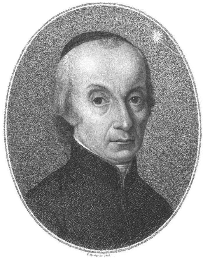
Figure: Giuseppe Piazzi (1746-1826) was an Italian Catholic priest and an astronomer. Jesuits had been closely involved in education, following their surpression in the Kingdom of Naples and Sicily, Piazzi was recruited as part of a drive to revitalize the University of Palermo. His funding was from King Ferdinand I and enabled him to buy high quality instruments from London.
Figure: Announcement of Giuseppe Piazzi’s discovery in the “Monthly Magazine” (also known as the British Register). This announcement is made in August 1801, 7 months after Giuseppe Piazzi first observed Ceres.
The planet’s location was a prediction. It was a missing planet, other planets had been found through a formula, a law, that represented their distance from the sun: \[ a = 0.4 + 0.3 \times 2^m \] where \(m=-\infty, 0, 1, 2, \dots\).
import numpy as npm = np.asarray([-np.inf, 0, 1, 2, 3, 4, 5, 6])
index = np.asarray(range(len(m)))
planets = ['Mercury', 'Venus', 'Earth', 'Mars', '*', 'Jupiter', 'Saturn', 'Uranus']
a = 0.5 + 0.3*2**mFigure: The Titius-Bode law was a relatively obscure empirical observation about how the planets are distributed across the solar system. It became well known after the discovery of Uranus by Herschel in 1781 which was found at the location the law predicts for the 8th planet.
When this law was published it fitted all known planets: Mercury, Venus, Earth, Mars, Jupiter and Saturn. Although there was a gap between the fourth and fifth planets (between Mars and Jupiter). In 1781 William Herschel discovered Uranus. It was in the position predicted by the formula. One of the originators of the formula, Johann Elert Bode urged astronomers to search for the missing planet, to be situated between Mars and Jupiter. Franz Xaver von Zach formed the United Astronomical Society, also known as the Celestial Police. But before the celestial police managed to start their search, Piazzi, without even knowing he was a member completed the search. Piazzi first observed the new planet in the early hours of January 1st 1801. He continued to observe it over the next 42 days. Initially he thought it may be a comet, but as he watched it he became convinced he’d found a planet. The international search was over before it started.
Unfortunately, there was a problem. Once he’d found the planet, Piazzi promptly lost it. Piazzi was keen not just to discover the planet, but to to be known as the determiner of its orbit. He took observations across the months of January and February, working to find the orbit. Unfortunately, he was unable to pin it down. He became ill, and by the time the dat awas revealed to the wider community through von Zach’s journal, Monatlicher Correspondenz, the new planet had been lost behind the sun.
Figure: Page from the publication Monatliche Correspondenz that shows Piazzi’s observations of the new planet Piazzi (n.d.) .
cmd = install_command('pods')%system {cmd}import urllib.requesturllib.request.urlretrieve('http://server3.sky-map.org/imgcut?survey=DSS2&img_id=all&angle=4&ra=3.5&de=17.25&width=1600&height=1600&projection=tan&interpolation=bicubic&jpeg_quality=0.8&output_type=png','ceres-sky-background.png')import podsdata = pods.datasets.ceres()
right_ascension = data['data']['Gerade Aufstig in Zeit']
declination = data['data']['Nordlich Abweich']Figure: Plot of the declination and right ascension that Piazzi recorded as Ceres passed through the sky in 1800. Gaps are evenings where Piazzi was unable to make an observation.
Piazzi was able to attempt to predict the orbit because of Kepler’s laws of planetary motion. Johannes Kepler had outlined the way in which planets move according to elliptical shapes, and comets move according to parabolic shapes.
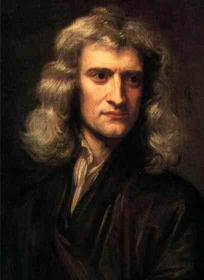
Figure: Godfrey Kneller portrait of Isaac Newton
Later Isaac Newton was able to describe the underlying laws of motion that underpinned Kepler’s laws. This was the enlightenment. An age of science and reason driven by reductionist approaches to the natural world. The enlightenment scientists were able to read and understand each other’s work through the invention of the printing press. Kepler died in 1630, 12 years before Newton was born in 1642. But Kepler’s ideas were able to influence Newton and his peers, and the understanding of gravity became an objective of the nascent Royal Society.
The sharing of information in printed form had evolved by the time of Piazzi, and the collected discoveries of the astronomic world were being shared in Franz von Zach’s monthly journal. It was here that Piazzi’s observations were eventually published, some 7 months after the planet was lost.
It was also here that a young German mathematician read about the international hunt for the lost planet. Carl Friedrich Gauss was a 23-year-old mathematician working from Göttingen. He combined Kepler’s laws with Piazzi’s data to make predictions about where the planet would be found. In doing so, he also developed the method of least squares, and incredibly was able to fit the relatively complex model to the data with a high enough degree of accuracy that astronomers were able to look to the skies to try to recover the planet.
Almost exactly one year after it was lost, Ceres was recovered by Franz von Zach. Gauss had combined model with data to make a prediction and in doing so a new planet was discovered Gauss (1802).
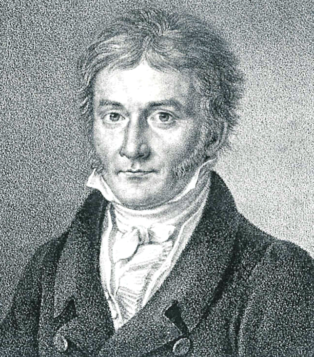
Figure: Carl Friedrich Gauss in 1828. He became internationally famous 27 years earlier for recovering the planet Ceres with a mathematical prediction.
It is this combination of model and data that underpins machine learning but notice that here it has also been delivered through a mechanistic understanding of the way the planets move. This understanding is derived from natural laws that are explicitly incorporated into the model. Kepler’s laws derive from Newton’s mathematical representation of gravity.
But there was a problem. The laws don’t precisely fit the data.
Figure: Gauss’s prediction of Ceres’s orbit as published in Franz von Zach’s Monatliche Correspondenz. He gives the location where the planet may be found, and then some mathematics for making other predictions. He doesn’t share his method, and this later leads to a priority dispute with Legendre around least-squares, which Gauss used to form the fit

Figure: Piazzi achieved his glory after the planet was discovered. Ceres is an agricultural god (in Greek tradition Demeter). She was associated with Sicily, where Piazzi was working when he made the discovery.
Unfortunately, the story doesn’t end so well for the Titsius-Bode law. In 1846 Neptune was discovered, not in the place predicted by the law (it should be closer to where Pluto was eventually found). And Ceres was found to be merely the largest object in the asteroid belt. It was recategorized as a Dwarf planet.
|
|
|
|
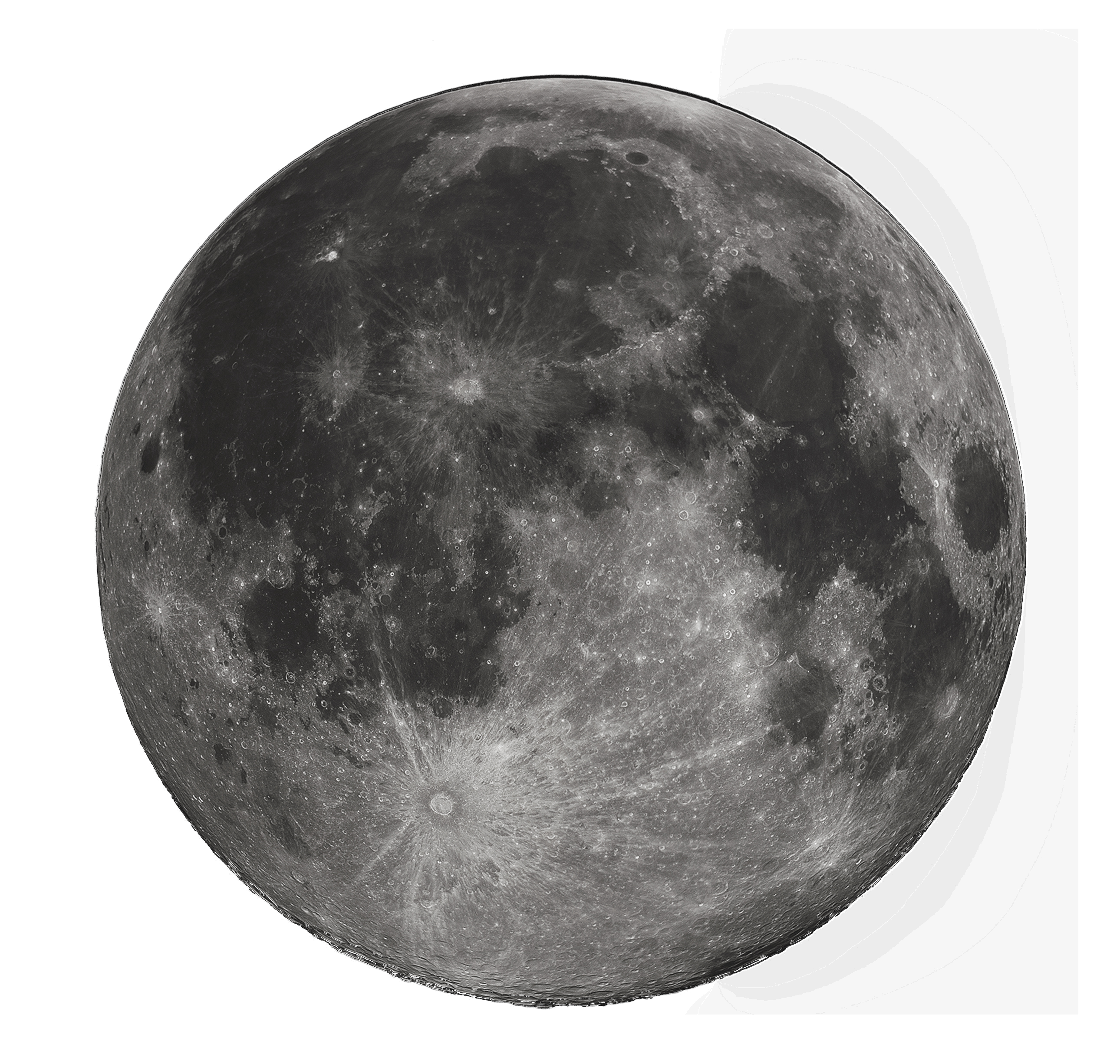
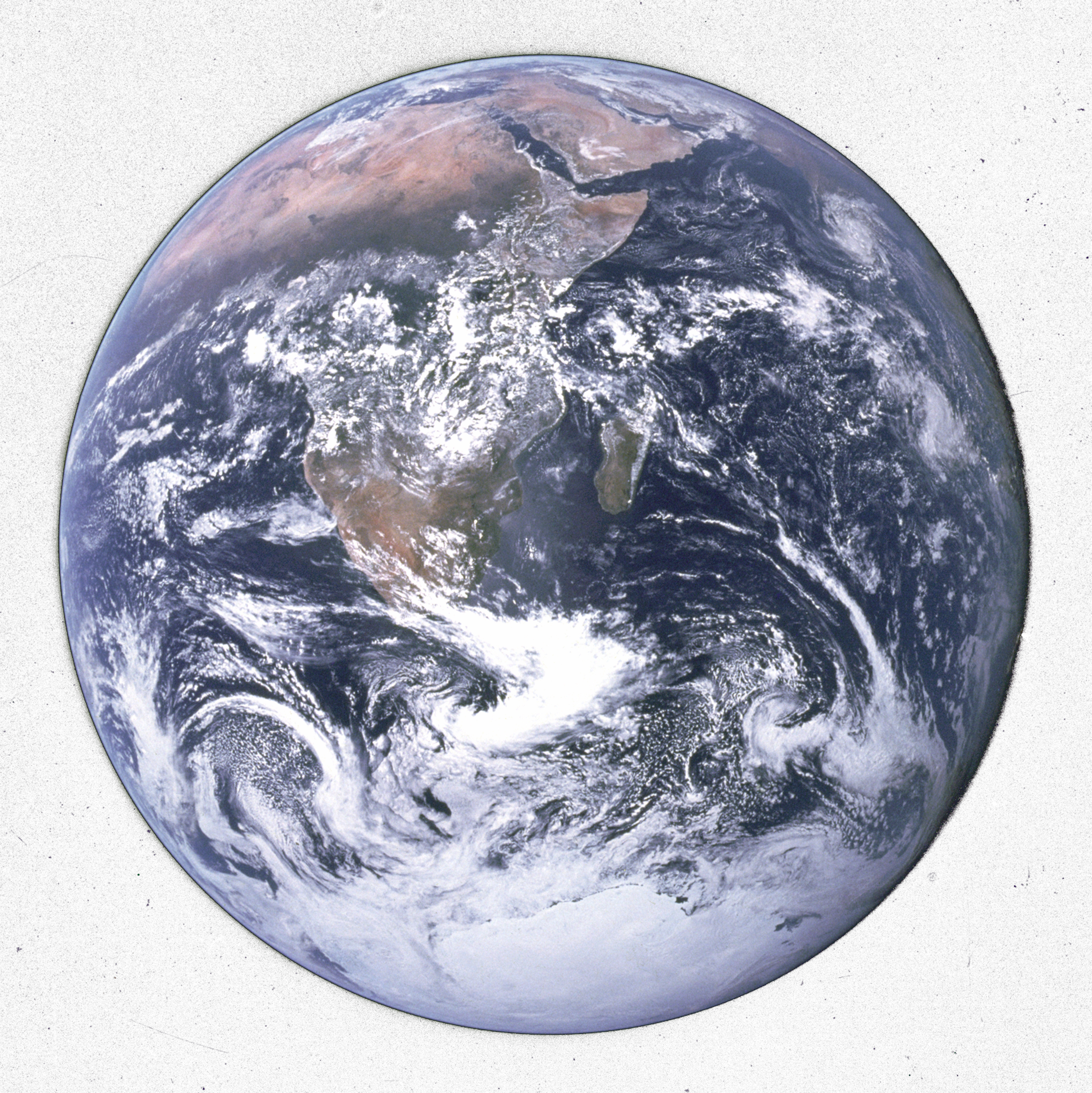
Figure: The surface area of Ceres is 2,850,000 square kilometers, it’s a little bigger than Greenland, but quite a lot colder. The moon is about 27% of the width of the Earth. Ceres is 7% of the width of the Earth.
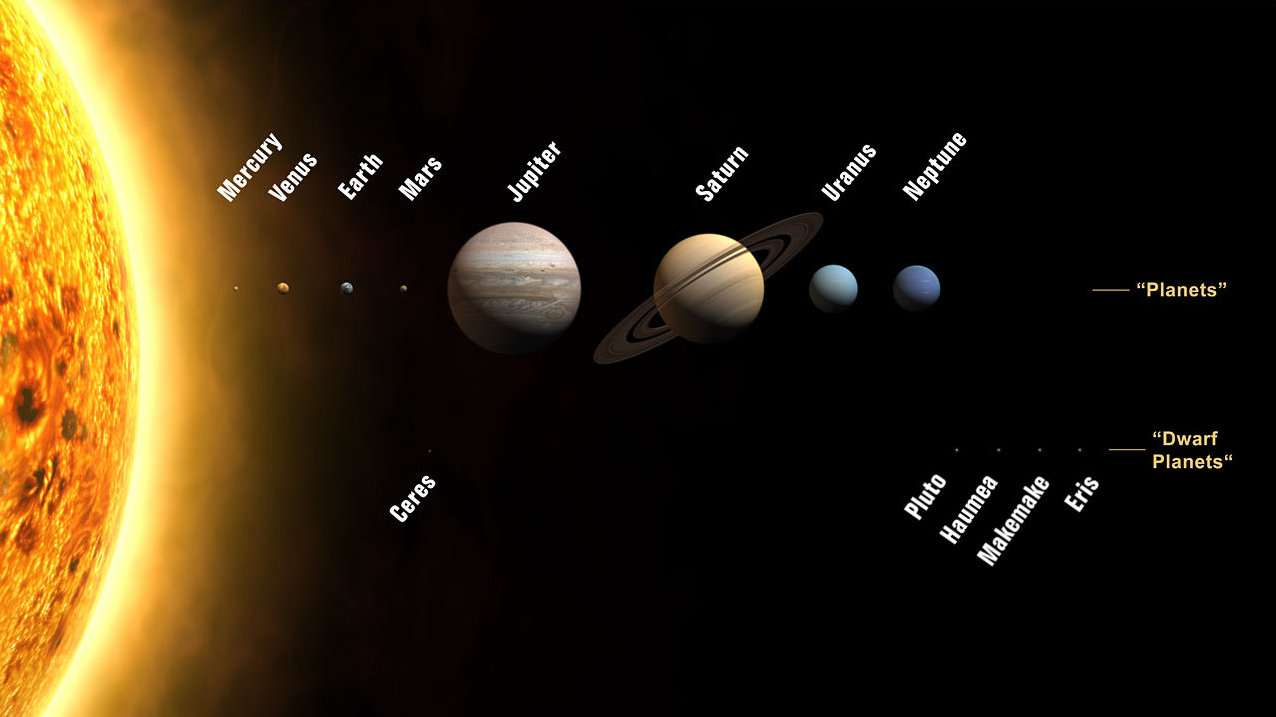
Figure: The location of Ceres as ordered in the solar system. While no longer a planet, Ceres is the unique Dwarf Planet in the inner solar system. This image from http://upload.wikimedia.org/wikipedia/commons/c/c4/Planets2008.jpg
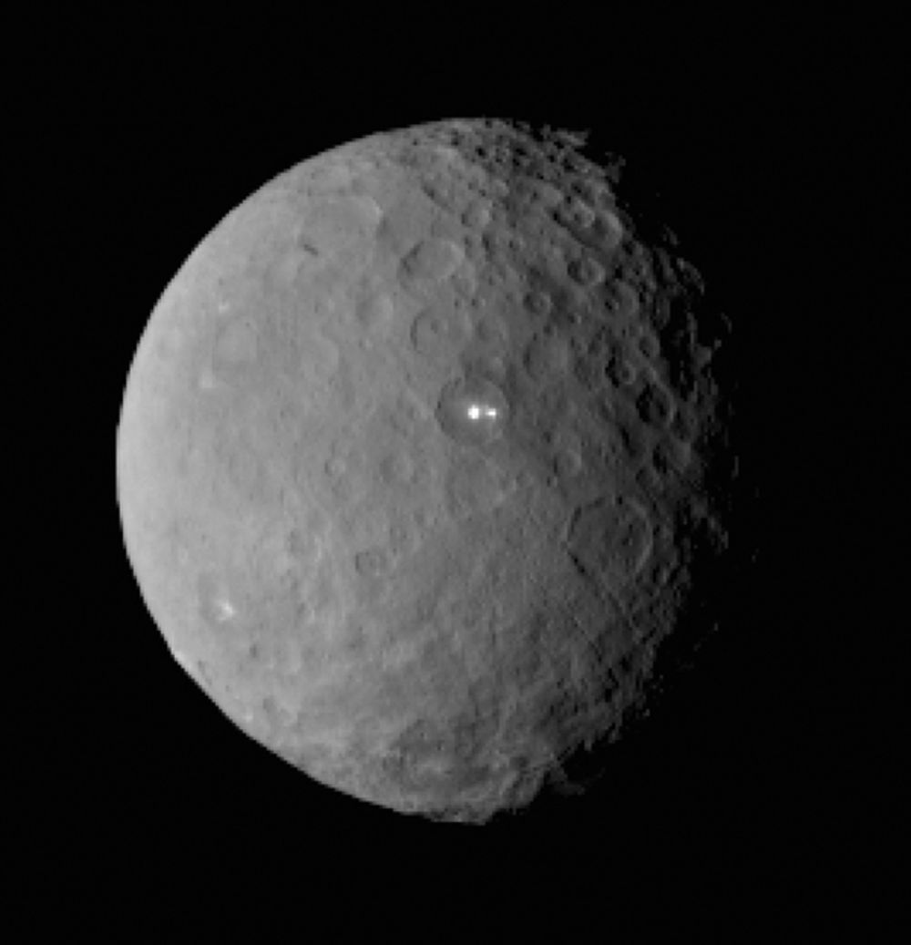
Figure: Ceres as photographed by the Dawn Mission. The photo highlights Ceres’s ‘bright spots’ which are thought to be a material with a high level of reflection (perhaps ice or salt). This image from http://www.popsci.com/sites/popsci.com/files/styles/large_1x_/public/dawn-two-bright-spots.jpg?itok=P5oeSRrc
Overdetermined System
The challenge with a linear model is that it has two unknowns, \(m\), and \(c\). Observing data allows us to write down a system of simultaneous linear equations. So, for example if we observe two data points, the first with the input value, \(x_1 = 1\) and the output value, \(y_1 =3\) and a second data point, \(x= 3\), \(y=1\), then we can write two simultaneous linear equations of the form.
point 1: \(x= 1\), \(y=3\) \[ 3 = m + c \] point 2: \(x= 3\), \(y=1\) \[ 1 = 3m + c \]
The solution to these two simultaneous equations can be represented graphically as
Figure: The solution of two linear equations represented as the fit of a straight line through two data
The challenge comes when a third data point is observed, and it doesn’t fit on the straight line.
point 3: \(x= 2\), \(y=2.5\) \[ 2.5 = 2m + c \]
Figure: A third observation of data is inconsistent with the solution dictated by the first two observations
Now there are three candidate lines, each consistent with our data.
Figure: Three solutions to the problem, each consistent with two points of the three observations
This is known as an overdetermined system because there are more data than we need to determine our parameters. The problem arises because the model is a simplification of the real world, and the data we observe is therefore inconsistent with our model.
Pierre-Simon Laplace
The solution was proposed by Pierre-Simon Laplace. His idea was to accept that the model was an incomplete representation of the real world, and the way it was incomplete is unknown. His idea was that such unknowns could be dealt with through probability.
Pierre-Simon Laplace
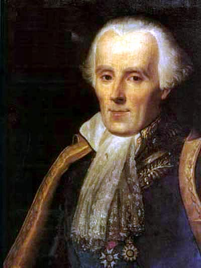
Figure: Pierre-Simon Laplace 1749-1827.
Famously, Laplace considered the idea of a deterministic Universe, one in which the model is known, or as the below translation refers to it, “an intelligence which could comprehend all the forces by which nature is animated.” He speculates on an “intelligence” that can submit this vast data to analysis and propsoses that such an entity would be able to predict the future.
Given for one instant an intelligence which could comprehend all the forces by which nature is animated and the respective situation of the beings who compose it—an intelligence sufficiently vast to submit these data to analysis—it would embrace in the same formulate the movements of the greatest bodies of the universe and those of the lightest atom; for it, nothing would be uncertain and the future, as the past, would be present in its eyes.
This notion is known as Laplace’s demon or Laplace’s superman.
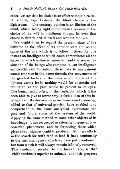
Figure: Laplace’s determinsim in English translation.
Laplace’s Gremlin
Unfortunately, most analyses of his ideas stop at that point, whereas his real point is that such a notion is unreachable. Not so much superman as strawman. Just three pages later in the “Philosophical Essay on Probabilities” (Laplace, 1814), Laplace goes on to observe:
The curve described by a simple molecule of air or vapor is regulated in a manner just as certain as the planetary orbits; the only difference between them is that which comes from our ignorance.
Probability is relative, in part to this ignorance, in part to our knowledge.
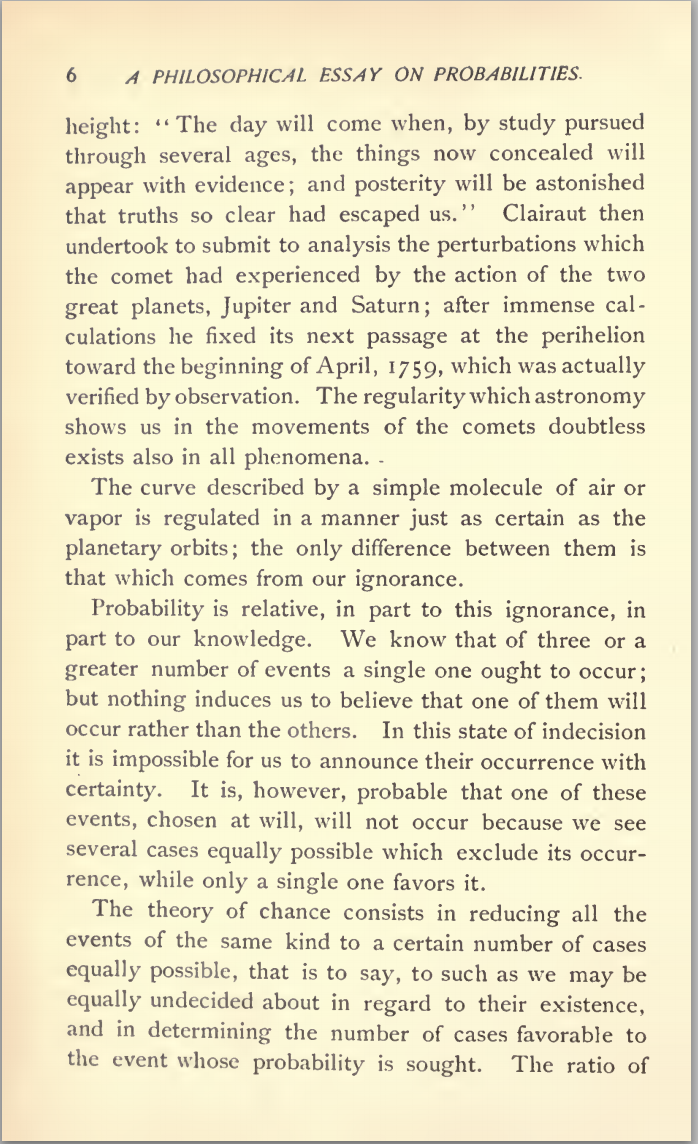
Figure: To Laplace, determinism is a strawman. Ignorance of mechanism and data leads to uncertainty which should be dealt with through probability.
In other words, we can never make use of the idealistic deterministic Universe due to our ignorance about the world, Laplace’s suggestion, and focus in this essay is that we turn to probability to deal with this uncertainty. This is also our inspiration for using probability in machine learning. This is the true message of Laplace’s essay, not determinism, but the gremlin of uncertainty that emerges from our ignorance.
The “forces by which nature is animated” is our model, the “situation of beings that compose it” is our data and the “intelligence sufficiently vast enough to submit these data to analysis” is our compute. The fly in the ointment is our ignorance about these aspects. And probability is the tool we use to incorporate this ignorance leading to uncertainty or doubt in our predictions.
Latent Variables
Laplace’s concept was that the reason that the data doesn’t match up to the model is because of unconsidered factors, and that these might be well represented through probability densities. He tackles the challenge of the unknown factors by adding a variable, \(\epsilon\), that represents the unknown. In modern parlance we would call this a latent variable. But in the context Laplace uses it, the variable is so common that it has other names such as a “slack” variable or the noise in the system.
point 1: \(x= 1\), \(y=3\) \[ 3 = m + c + \epsilon_1 \] point 2: \(x= 3\), \(y=1\) \[ 1 = 3m + c + \epsilon_2 \] point 3: \(x= 2\), \(y=2.5\) \[ 2.5 = 2m + c + \epsilon_3 \]
Laplace’s trick has converted the overdetermined system into an underdetermined system. He has now added three variables, \(\{\epsilon_i\}_{i=1}^3\), which represent the unknown corruptions of the real world. Laplace’s idea is that we should represent that unknown corruption with a probability distribution.
A Probabilistic Process
However, it was left to an admirer of Laplace to develop a practical probability density for that purpose. It was Carl Friedrich Gauss who suggested that the Gaussian density (which at the time was unnamed!) should be used to represent this error.
The result is a noisy function, a function which has a deterministic part, and a stochastic part. This type of function is sometimes known as a probabilistic or stochastic process, to distinguish it from a deterministic process.
Brownian Motion and Wiener
Robert Brown was a botanist who was studying plant pollen in 1827 when he noticed a trembling motion of very small particles contained within cavities within the pollen. He worked hard to eliminate the potential source of the movement by exploring other materials where he found it to be continuously present. Thus, the movement was not associated, as he originally thought, with life.
In 1905 Albert Einstein produced the first mathematical explanation of the phenomenon. This can be seen as our first model of a ‘curve of a simple molecule of air.’ To model the phenomenon Einstein introduced stochasticity to a differential equation. The particles were being peppered with high-speed water molecules, that was triggering the motion. Einstein modelled this as a stochastic process.
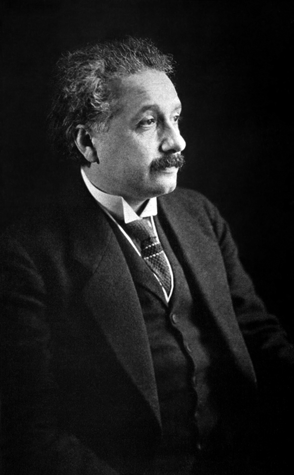
Figure: Albert Einstein’s 1905 paper on Brownian motion introduced stochastic differential equations which can be used to model the ‘curve of a simple molecule of air.’
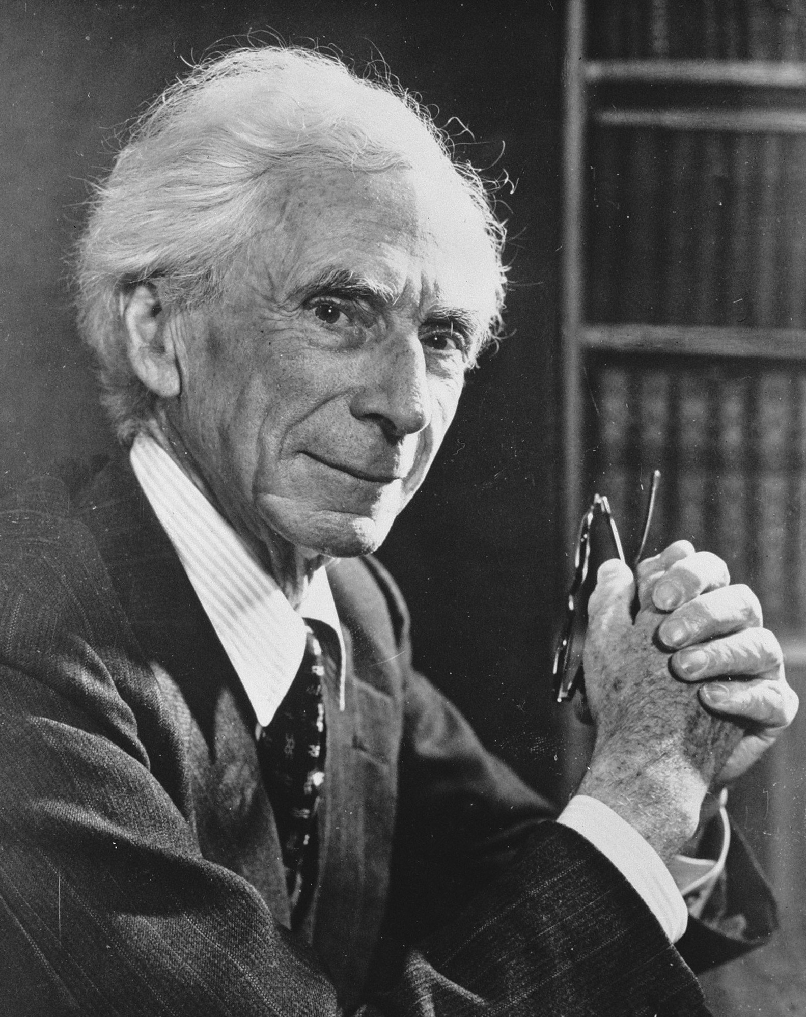
Norbert Wiener was a child prodigy, whose father had schooled him in philosophy. He was keen to have his son work with the leading philosophers of the age, so at the age of 18 Wiener arrived in Cambridge (already with a PhD). He was despatched to study with Bertrand Russell but Wiener and Russell didn’t get along. Wiener wasn’t persuaded by Russell’s ideas for theories of knowledge through logic. He was more aligned with Laplace and his desire for a theory of ignorance. In is autobiography he relates it as the first thing he could see his father was proud of (at around the age of 10 or 11) (Wiener, 1953).
|
|
|
Figure: Bertrand Russell (1872-1970), Albert Einstein (1879-1955), Norbert Wiener, (1894-1964)
But Russell (despite also not getting along well with Wiener) introduced Wiener to Einstein’s works, and Wiener also met G. H. Hardy. He left Cambridge for Göttingen where he studied with Hilbert. He developed the underlying mathematics for proving the existence of the solutions to Einstein’s equation, which are now known as Wiener processes.
Figure: Brownian motion of a large particle in a group of smaller particles. The movement is known as a Wiener process after Norbert Wiener.
|
|
|
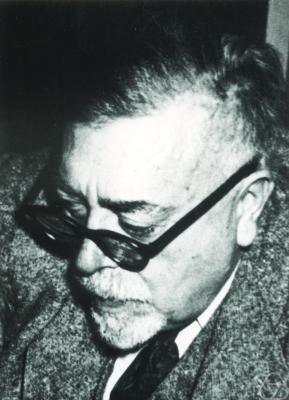
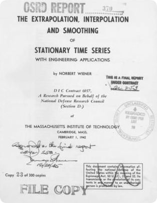
Figure: Norbert Wiener (1894 - 1964). Founder of cybernetics and the information era. He used Gibbs’s ideas to develop a “theory of ignorance” that he deployed in early communication. On the right is Wiener’s wartime report that used stochastic processes in forecasting with applications in radar control (image from Coales and Kane (2014)).
Wiener himself used the processes in his work. He was focused on mathematical theories of communication. Between the world wars he was based at Massachusetts Institute of Technology where the burgeoning theory of electrical engineering was emerging, with a particular focus on communication lines. Winer developed theories of communication that used Gibbs’s entropy to encode information. He also used the ideas behind the Wiener process for developing tracking methods for radar systems in the second world war. These processes are what we know of now as Gaussian processes (Wiener (1949)).
|
|
|
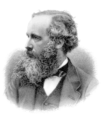
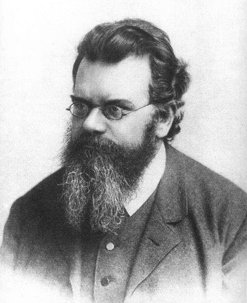
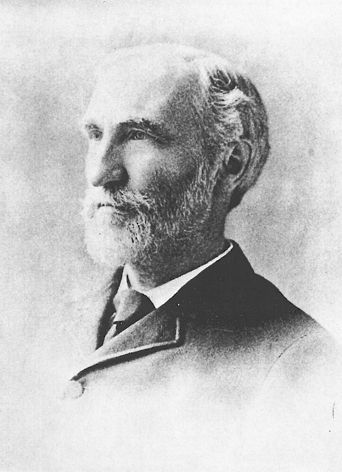
Figure: James Clerk Maxwell (1831-1879), Ludwig Boltzmann (1844-1906) Josiah Willard Gibbs (1839-1903)
Entropy Billiards
Figure: Bernoulli’s simple kinetic models of gases assume that the molecules of air operate like billiard balls.
Underdetermined System
What about the situation where you have more parameters than data in your simultaneous equation? This is known as an underdetermined system. In fact, this set up is in some sense easier to solve, because we don’t need to think about introducing a slack variable (although it might make a lot of sense from a modelling perspective to do so).
The way Laplace proposed resolving an overdetermined system, was to introduce slack variables, \(\epsilon_i\), which needed to be estimated for each point. The slack variable represented the difference between our actual prediction and the true observation. This is known as the residual. By introducing the slack variable, we now have an additional \(n\) variables to estimate, one for each data point, \(\{\epsilon_i\}\). This turns the overdetermined system into an underdetermined system. Introduction of \(n\) variables, plus the original \(m\) and \(c\) gives us \(n+2\) parameters to be estimated from \(n\) observations, which makes the system underdetermined. However, we then made a probabilistic assumption about the slack variables, we assumed that the slack variables were distributed according to a probability density. And for the moment we have been assuming that density was the Gaussian, \[\epsilon_i \sim \mathscr{N}\left(0,\sigma^2\right),\] with zero mean and variance \(\sigma^2\).
The follow up question is whether we can do the same thing with the parameters. If we have two parameters and only one unknown, can we place a probability distribution over the parameters as we did with the slack variables? The answer is yes.
Underdetermined System
Figure: An underdetermined system can be fit by considering uncertainty. Multiple solutions are consistent with one specified point.
Probabilities
We are now going to do some simple review of probabilities and use this review to explore some aspects of our data.
A probability distribution expresses uncertainty about the outcome of an event. We often encode this uncertainty in a variable. So if we are considering the outcome of an event, \(Y\), to be a coin toss, then we might consider \(Y=1\) to be heads and \(Y=0\) to be tails. We represent the probability of a given outcome with the notation: \[ P(Y=1) = 0.5 \] The first rule of probability is that the probability must normalize. The sum of the probability of all events must equal 1. So if the probability of heads (\(Y=1\)) is 0.5, then the probability of tails (the only other possible outcome) is given by \[ P(Y=0) = 1-P(Y=1) = 0.5 \]
Probabilities are often defined as the limit of the ratio between the number of positive outcomes (e.g. heads) given the number of trials. If the number of positive outcomes for event \(y\) is denoted by \(n\) and the number of trials is denoted by \(N\) then this gives the ratio \[ P(Y=y) = \lim_{N\rightarrow \infty}\frac{n_y}{N}. \] In practice we never get to observe an event infinite times, so rather than considering this we often use the following estimate \[ P(Y=y) \approx \frac{n_y}{N}. \]
Nigeria NMIS Data
As an example data set we will use Nigerian Millennium Development Goals Information System Health Facility (The Office of the Senior Special Assistant to the President on the Millennium Development Goals (OSSAP-MDGs) and Columbia University, 2014). It can be found here https://energydata.info/dataset/nigeria-nmis-education-facility-data-2014.
Taking from the information on the site,
The Nigeria MDG (Millennium Development Goals) Information System – NMIS health facility data is collected by the Office of the Senior Special Assistant to the President on the Millennium Development Goals (OSSAP-MDGs) in partner with the Sustainable Engineering Lab at Columbia University. A rigorous, geo-referenced baseline facility inventory across Nigeria is created spanning from 2009 to 2011 with an additional survey effort to increase coverage in 2014, to build Nigeria’s first nation-wide inventory of health facility. The database includes 34,139 health facilities info in Nigeria.
The goal of this database is to make the data collected available to planners, government officials, and the public, to be used to make strategic decisions for planning relevant interventions.
For data inquiry, please contact Ms. Funlola Osinupebi, Performance Monitoring & Communications, Advisory Power Team, Office of the Vice President at funlola.osinupebi@aptovp.org
To learn more, please visit http://csd.columbia.edu/2014/03/10/the-nigeria-mdg-information-system-nmis-takes-open-data-further/
Suggested citation: Nigeria NMIS facility database (2014), the Office of the Senior Special Assistant to the President on the Millennium Development Goals (OSSAP-MDGs) & Columbia University
For ease of use we’ve packaged this data set in the pods library
data = pods.datasets.nigeria_nmis()['Y']
data.head()
Alternatively, you can access the data directly with the following commands.
import urllib.request
urllib.request.urlretrieve('https://energydata.info/dataset/f85d1796-e7f2-4630-be84-79420174e3bd/resource/6e640a13-cab4-457b-b9e6-0336051bac27/download/healthmopupandbaselinenmisfacility.csv', 'healthmopupandbaselinenmisfacility.csv')

import pandas as pd
data = pd.read_csv('healthmopupandbaselinenmisfacility.csv')
Once it is loaded in the data can be summarized using the describe method in pandas.
data.describe()We can also find out the dimensions of the dataset using the shape property.
data.shapeDataframes have different functions that you can use to explore and understand your data. In python and the Jupyter notebook it is possible to see a list of all possible functions and attributes by typing the name of the object followed by .<Tab> for example in the above case if we type data.<Tab> it show the columns available (these are attributes in pandas dataframes) such as num_nurses_fulltime, and also functions, such as .describe().
For functions we can also see the documentation about the function by following the name with a question mark. This will open a box with documentation at the bottom which can be closed with the x button.
data.describe?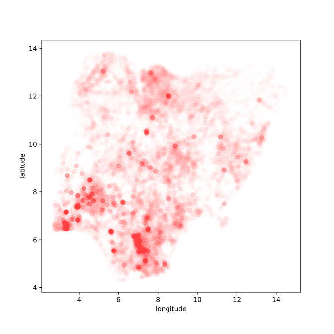
Figure: Location of the over thirty-four thousand health facilities registered in the NMIS data across Nigeria. Each facility plotted according to its latitude and longitude.
Exploring the NMIS Data
The NMIS facility data is stored in an object known as a ‘data frame.’ Data frames come from the statistical family of programming languages based on S, the most widely used of which is R. The data frame gives us a convenient object for manipulating data. The describe method summarizes which columns there are in the data frame and gives us counts, means, standard deviations and percentiles for the values in those columns. To access a column directly we can write
print(data['num_doctors_fulltime'])
#print(data['num_nurses_fulltime'])
This shows the number of doctors per facility, number of nurses and number of community health workers (CHEWS). We can plot the number of doctors against the number of nurses as follows.
import matplotlib.pyplot as plt # this imports the plotting library in python_ = plt.plot(data['num_doctors_fulltime'], data['num_nurses_fulltime'], 'rx')You may be curious what the arguments we give to plt.plot are for, now is the perfect time to look at the documentation
plt.plot?We immediately note that some facilities have a lot of nurses, which prevent’s us seeing the detail of the main number of facilities. First lets identify the facilities with the most nurses.
data[data['num_nurses_fulltime']>100]Here we are using the command data['num_nurses_fulltime']>100 to index the facilities in the pandas data frame which have over 100 nurses. To sort them in order we can also use the sort command. The result of this command on its own is a data Series of True and False values. However, when it is passed to the data data frame it returns a new data frame which contains only those values for which the data series is True. We can also sort the result. To sort the result by the values in the num_nurses_fulltime column in descending order we use the following command.
data[data['num_nurses_fulltime']>100].sort_values(by='num_nurses_fulltime', ascending=False)We now see that the ‘University of Calabar Teaching Hospital’ is a large outlier with 513 nurses. We can try and determine how much of an outlier by histograming the data.
Plotting the Data
data['num_nurses_fulltime'].hist(bins=20) # histogram the data with 20 bins.
plt.title('Histogram of Number of Nurses')
We can’t see very much here. Two things are happening. There are so many facilities with zero or one nurse that we don’t see the histogram for hospitals with many nurses. We can try more bins and using a log scale on the \(y\)-axis.
data['num_nurses_fulltime'].hist(bins=100) # histogram the data with 20 bins.
plt.title('Histogram of Number of Nurses')
ax = plt.gca()
ax.set_yscale('log')
Let’s try and see how the number of nurses relates to the number of doctors.
fig, ax = plt.subplots(figsize=(10, 7))
ax.plot(data['num_doctors_fulltime'], data['num_nurses_fulltime'], 'rx')
ax.set_xscale('log') # use a logarithmic x scale
ax.set_yscale('log') # use a logarithmic Y scale
# give the plot some titles and labels
plt.title('Number of Nurses against Number of Doctors')
plt.ylabel('number of nurses')
plt.xlabel('number of doctors')
Note a few things. We are interacting with our data. In particular, we are replotting the data according to what we have learned so far. We are using the progamming language as a scripting language to give the computer one command or another, and then the next command we enter is dependent on the result of the previous. This is a very different paradigm to classical software engineering. In classical software engineering we normally write many lines of code (entire object classes or functions) before compiling the code and running it. Our approach is more similar to the approach we take whilst debugging. Historically, researchers interacted with data using a console. A command line window which allowed command entry. The notebook format we are using is slightly different. Each of the code entry boxes acts like a separate console window. We can move up and down the notebook and run each part in a different order. The state of the program is always as we left it after running the previous part.
Probability and the NMIS Data
Let’s use the sum rule to compute the estimate the probability that a facility has more than two nurses.
large = (data.num_nurses_fulltime>2).sum()  # number of positive outcomes (in sum True counts as 1, False counts as 0)
total_facilities = data.num_nurses_fulltime.count()

prob_large = float(large)/float(total_facilities)
print("Probability of number of nurses being greather than 2 is:", prob_large)
Conditioning
When predicting whether a coin turns up head or tails, we might think that this event is independent of the year or time of day. If we include an observation such as time, then in a probability this is known as condtioning. We use this notation, \(P(Y=y|X=x)\), to condition the outcome on a second variable (in this case the number of doctors). Or, often, for a shorthand we use \(P(y|x)\) to represent this distribution (the \(Y=\) and \(X=\) being implicit). If two variables are independent then we find that \[ P(y|x) = p(y). \] However, we might believe that the number of nurses is dependent on the number of doctors. For this we can try estimating \(P(Y>2 | X>1)\) and compare the result, for example to \(P(Y>2|X\leq 1)\) using our empirical estimate of the probability.
large = ((data.num_nurses_fulltime>2) & (data.num_doctors_fulltime>1)).sum()
total_large_doctors = (data.num_doctors_fulltime>1).sum()
prob_both_large = large/total_large_doctors
print("Probability of number of nurses being greater than 2 given number of doctors is greater than 1 is:", prob_both_large)
Exercise 1
Write code that prints out the probability of nurses being greater than 2 for different numbers of doctors.
Make sure the plot is included in this notebook file (the Jupyter magic command %matplotlib inline we ran above will do that for you, it only needs to be run once per file).
| Terminology | Mathematical notation | Description |
|---|---|---|
| joint | \(P(X=x, Y=y)\) | prob. that X=x and Y=y |
| marginal | \(P(X=x)\) | prob. that X=x regardless of Y |
| conditional | \(P(X=x\vert Y=y)\) | prob. that X=x given that Y=y |
A Pictorial Definition of Probability
Figure: Diagram representing the different probabilities, joint, marginal and conditional. This diagram was inspired by lectures given by Christopher Bishop.
Definition of probability distributions
| Terminology | Definition | Probability Notation |
|---|---|---|
| Joint Probability | \(\lim_{N\rightarrow\infty}\frac{n_{X=3,Y=4}}{N}\) | \(P\left(X=3,Y=4\right)\) |
| Marginal Probability | \(\lim_{N\rightarrow\infty}\frac{n_{X=5}}{N}\) | \(P\left(X=5\right)\) |
| Conditional Probability | \(\lim_{N\rightarrow\infty}\frac{n_{X=3,Y=4}}{n_{Y=4}}\) | \(P\left(X=3\vert Y=4\right)\) |
Notational Details
Typically we should write out \(P\left(X=x,Y=y\right)\), but in practice we often shorten this to \(P\left(x,y\right)\). This looks very much like we might write a multivariate function, e.g. \[ f\left(x,y\right)=\frac{x}{y}, \] but for a multivariate function \[ f\left(x,y\right)\neq f\left(y,x\right). \] However, \[ P\left(x,y\right)=P\left(y,x\right) \] because \[ P\left(X=x,Y=y\right)=P\left(Y=y,X=x\right). \] Sometimes I think of this as akin to the way in Python we can write ‘keyword arguments’ in functions. If we use keyword arguments, the ordering of arguments doesn’t matter.
We’ve now introduced conditioning and independence to the notion of probability and computed some conditional probabilities on a practical example The scatter plot of deaths vs year that we created above can be seen as a joint probability distribution. We represent a joint probability using the notation \(P(Y=y, X=x)\) or \(P(y, x)\) for short. Computing a joint probability is equivalent to answering the simultaneous questions, what’s the probability that the number of nurses was over 2 and the number of doctors was 1? Or any other question that may occur to us. Again we can easily use pandas to ask such questions.
num_doctors = 1
large = (data.num_nurses_fulltime[data.num_doctors_fulltime==num_doctors]>2).sum()
total_facilities = data.num_nurses_fulltime.count() # this is total number of films
prob_large = float(large)/float(total_facilities)
print("Probability of nurses being greater than 2 and number of doctors being", num_doctors, "is:", prob_large)
The Product Rule
This number is the joint probability, \(P(Y, X)\) which is much smaller than the conditional probability. The number can never be bigger than the conditional probabililty because it is computed using the product rule. \[ p(Y=y, X=x) = p(Y=y|X=x)p(X=x) \] and \[p(X=x)\] is a probability distribution, which is equal or less than 1, ensuring the joint distribution is typically smaller than the conditional distribution.
The product rule is a fundamental rule of probability, and you must remember it! It gives the relationship between the two questions: 1) What’s the probability that a facility has over two nurses and one doctor? and 2) What’s the probability that a facility has over two nurses given that it has one doctor?
In our shorter notation we can write the product rule as \[ p(y, x) = p(y|x)p(x) \] We can see the relation working in practice for our data above by computing the different values for \(x=1\).
num_doctors=1
num_nurses=2
p_x = float((data.num_doctors_fulltime==num_doctors).sum())/float(data.num_doctors_fulltime.count())
p_y_given_x = float((data.num_nurses_fulltime[data.num_doctors_fulltime==num_doctors]>num_nurses).sum())/float((data.num_doctors_fulltime==num_doctors).sum())
p_y_and_x = float((data.num_nurses_fulltime[data.num_doctors_fulltime==num_doctors]>num_nurses).sum())/float(data.num_nurses_fulltime.count())

print("P(x) is", p_x)
print("P(y|x) is", p_y_given_x)
print("P(y,x) is", p_y_and_x)
The Sum Rule
The other fundamental rule of probability is the sum rule this tells us how to get a marginal distribution from the joint distribution. Simply put it says that we need to sum across the value we’d like to remove. \[ P(Y=y) = \sum_{x} P(Y=y, X=x) \] Or in our shortened notation \[ P(y) = \sum_{x} P(y, x) \]
Exercise 2
Write code that computes \(P(y)\) by adding \(P(y, x)\) for all values of \(x\).
Bayes’ Rule
Bayes’ rule is a very simple rule, it’s hardly worth the name of a rule at all. It follows directly from the product rule of probability. Because \(P(y, x) = P(y|x)P(x)\) and by symmetry \(P(y,x)=P(x,y)=P(x|y)P(y)\) then by equating these two equations and dividing through by \(P(y)\) we have \[ P(x|y) = \frac{P(y|x)P(x)}{P(y)} \] which is known as Bayes’ rule (or Bayes’s rule, it depends how you choose to pronounce it). It’s not difficult to derive, and its importance is more to do with the semantic operation that it enables. Each of these probability distributions represents the answer to a question we have about the world. Bayes rule (via the product rule) tells us how to invert the probability.
Further Reading
- Probability distributions: page 12–17 (Section 1.2) of Bishop (2006)
Exercises
- Exercise 1.3 of Bishop (2006)
Probabilities for Extracting Information from Data
What use is all this probability in data science? Let’s think about how we might use the probabilities to do some decision making. Let’s look at the information data.
data.columnsExercise 3
Now we see we have several additional features. Let’s assume we want to predict maternal_health_delivery_services. How would we go about doing it?
Using what you’ve learnt about joint, conditional and marginal probabilities, as well as the sum and product rule, how would you formulate the question you want to answer in terms of probabilities? Should you be using a joint or a conditional distribution? If it’s conditional, what should the distribution be over, and what should it be conditioned on?
Figure: MLAI Lecture 2 from 2012.
See probability review at end of slides for reminders.
For other material in Bishop read:
If you are unfamiliar with probabilities you should complete the following exercises:
Thanks!
For more information on these subjects and more you might want to check the following resources.
- company: Trent AI
- book: The Atomic Human
- twitter: @lawrennd
- podcast: The Talking Machines
- newspaper: Guardian Profile Page
- blog: http://inverseprobability.com
Further Reading
Section 2.2 (pg 41–53) of Rogers and Girolami (2011)
Section 2.4 (pg 55–58) of Rogers and Girolami (2011)
Section 2.5.1 (pg 58–60) of Rogers and Girolami (2011)
Section 2.5.3 (pg 61–62) of Rogers and Girolami (2011)
Probability densities: Section 1.2.1 (Pages 17-19) of Bishop (2006)
Expectations and Covariances: Section 1.2.2 (Pages 19–20) of Bishop (2006)
The Gaussian density: Section 1.2.4 (Pages 24-28) (don’t worry about material on bias) of Bishop (2006)
For material on information theory and KL divergence try Section 1.6 & 1.6.1 (pg 48 onwards) of Bishop (2006)
Exercises
Exercise 1.7 of Bishop (2006)
Exercise 1.8 of Bishop (2006)
Exercise 1.9 of Bishop (2006)
References
The logarithm of a number less than one is negative, for a number greater than one the logarithm is positive. So if odds are greater than evens (odds-on) the log-odds are positive, if the odds are less than evens (odds-against) the log-odds will be negative.↩︎