Linear Algebra and Regression
Neil Lawrence
Dedan Kimathi University, Nyeri, Kenya
Review
- Last time: Reviewed Objective Functions and gradient descent.
Regression Examples
- Predict a real value, \(y_i\) given some inputs \(\mathbf{ x}_i\).
- Predict quality of meat given spectral measurements (Tecator data).
- Radiocarbon dating, the C14 calibration curve: predict age given quantity of C14 isotope.
- Predict quality of different Go or Backgammon moves given expert rated training data.
Latent Variables
\(y= mx+ c + \epsilon\)
point 1: \(x= 1\), \(y=3\) \[ 3 = m + c + \epsilon_1 \]
point 2: \(x= 3\), \(y=1\) \[ 1 = 3m + c + \epsilon_2 \]
point 3: \(x= 2\), \(y=2.5\) \[ 2.5 = 2m + c + \epsilon_3 \]
A Probabilistic Process
Set the mean of Gaussian to be a function. \[ p\left(y_i|x_i\right)=\frac{1}{\sqrt{2\pi\sigma^2}}\exp \left(-\frac{\left(y_i-f\left(x_i\right)\right)^{2}}{2\sigma^2}\right). \]
This gives us a ‘noisy function.’
This is known as a stochastic process.
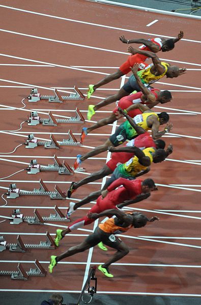
Olympic 100m Data
|
|
Olympic 100m Data
Sum of Squares Error
\[ E(\mathbf{ w}) = \sum_{i=1}^n \left(y_i - \mathbf{ x}_i^\top \mathbf{ w}\right)^2 \]
- Will recast with probabilistic motivation.
- First, reminder of Gaussian distribution.
Sum of Squares and Probability
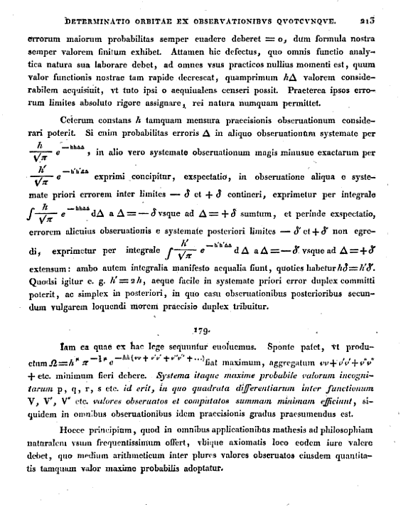
… It is clear, that for the product \(\Omega = h^\mu \pi^{-\frac{1}{2}\mu} e^{-hh(vv + v^\prime v^\prime + v^{\prime\prime} v^{\prime\prime} + \dots)}\) to be maximised the sum \(vv + v ^\prime v^\prime + v^{\prime\prime} v^{\prime\prime} + \text{etc}.\) ought to be minimized. Therefore, the most probable values of the unknown quantities \(p , q, r , s \text{etc}.\), should be that in which the sum of the squares of the differences between the functions \(V, V^\prime, V^{\prime\prime} \text{etc}\), and the observed values is minimized, for all observations of the same degree of precision is presumed.
The Gaussian Density
- Perhaps the most common probability density.
\[\begin{align} p(y| \mu, \sigma^2) & = \frac{1}{\sqrt{2\pi\sigma^2}}\exp\left(-\frac{(y- \mu)^2}{2\sigma^2}\right)\\& \buildrel\triangle\over = \mathscr{N}\left(y|\mu,\sigma^2\right) \end{align}\]
Gaussian Density
Gaussian Density
Two Important Gaussian Properties
Sum of Gaussians
\[y_i \sim \mathscr{N}\left(\mu_i,\sigma_i^2\right)\]
\[ \sum_{i=1}^{n} y_i \sim \mathscr{N}\left(\sum_{i=1}^n\mu_i,\sum_{i=1}^n\sigma_i^2\right) \]
(Aside: As sum increases, sum of non-Gaussian, finite variance variables is also Gaussian because of central limit theorem.)
Scaling a Gaussian
\[y\sim \mathscr{N}\left(\mu,\sigma^2\right)\]
\[wy\sim \mathscr{N}\left(w\mu,w^2 \sigma^2\right).\]
Laplace’s Idea
A Probabilistic Process
Set the mean of Gaussian to be a function.
\[p\left(y_i|x_i\right)=\frac{1}{\sqrt{2\pi\sigma^2}}\exp\left(-\frac{\left(y_i-f\left(x_i\right)\right)^{2}}{2\sigma^2}\right).\]
This gives us a ‘noisy function.’
This is known as a stochastic process.
Height as a Function of Weight
In the standard Gaussian, parameterized by mean and variance, make the mean a linear function of an input.
This leads to a regression model. \[ \begin{align*} y_i=&f\left(x_i\right)+\epsilon_i,\\ \epsilon_i \sim & \mathscr{N}\left(0,\sigma^2\right). \end{align*} \]
Assume \(y_i\) is height and \(x_i\) is weight.
Data Point Likelihood
Likelihood of an individual data point \[ p\left(y_i|x_i,m,c\right)=\frac{1}{\sqrt{2\pi \sigma^2}}\exp\left(-\frac{\left(y_i-mx_i-c\right)^{2}}{2\sigma^2}\right). \] Parameters are gradient, \(m\), offset, \(c\) of the function and noise variance \(\sigma^2\).
Data Set Likelihood
If the noise, \(\epsilon_i\) is sampled independently for each data point. Each data point is independent (given \(m\) and \(c\)). For independent variables: \[ p(\mathbf{ y}) = \prod_{i=1}^np(y_i) \] \[ p(\mathbf{ y}|\mathbf{ x}, m, c) = \prod_{i=1}^np(y_i|x_i, m, c) \]
For Gaussian
i.i.d. assumption \[ p(\mathbf{ y}|\mathbf{ x}, m, c) = \prod_{i=1}^n\frac{1}{\sqrt{2\pi \sigma^2}}\exp \left(-\frac{\left(y_i- mx_i-c\right)^{2}}{2\sigma^2}\right). \]
\[ p(\mathbf{ y}|\mathbf{ x}, m, c) = \frac{1}{\left(2\pi \sigma^2\right)^{\frac{n}{2}}}\exp\left(-\frac{\sum_{i=1}^n\left(y_i-mx_i-c\right)^{2}}{2\sigma^2}\right). \]
Log Likelihood Function
- Normally work with the log likelihood: \[\begin{aligned} L(m,c,\sigma^{2})= & -\frac{n}{2}\log 2\pi -\frac{n}{2}\log \sigma^2 \\& -\sum_{i=1}^{n}\frac{\left(y_i-mx_i-c\right)^{2}}{2\sigma^2}. \end{aligned}\]
Consistency of Maximum Likelihood
- If data was really generated according to probability we specified.
- Correct parameters will be recovered in limit as \(n\rightarrow \infty\).
Consistency of Maximum Likelihood
- This can be proven through sample based approximations (law of large numbers) of “KL divergences.”
- Mainstay of classical statistics (Wasserman, 2003).
Probabilistic Interpretation of Error Function
- Probabilistic Interpretation for Error Function is Negative Log Likelihood.
- Minimizing error function is equivalent to maximizing log likelihood.
Probabilistic Interpretation of Error Function
- Maximizing log likelihood is equivalent to maximizing the likelihood because \(\log\) is monotonic.
- Probabilistic interpretation: Minimizing error function is equivalent to maximum likelihood with respect to parameters.
Error Function
- Negative log likelihood leads to an error function \[\begin{aligned} E(m,c,\sigma^{2})= & \frac{n}{2}\log \sigma^2 \\& +\frac{1}{2\sigma^2}\sum _{i=1}^{n}\left(y_i-mx_i-c\right)^{2}.\end{aligned}\]
- Learning by minimising error function.
Sum of Squares Error
- Ignoring terms which don’t depend on \(m\) and \(c\) gives \[E(m, c) \propto \sum_{i=1}^n(y_i - f(x_i))^2\] where \(f(x_i) = mx_i + c\).
Sum of Squares Error
- This is recognised as the sum of squares error function.
- Commonly used and is closely associated with the Gaussian likelihood.
Reminder
- Two functions involved:
- Prediction function: \(f(x_i)\)
- Error, or Objective function: \(E(m, c)\)
- Error function depends on parameters through prediction function.
Mathematical Interpretation
- What is the mathematical interpretation?
- There is a cost function.
- It expresses mismatch between your prediction and reality. \[ E(m, c)=\sum_{i=1}^n\left(y_i - mx_i-c\right)^2 \]
- This is known as the sum of squares error.
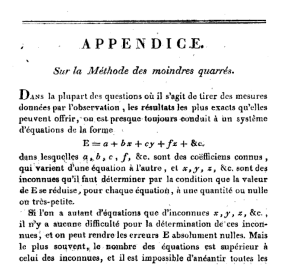
Legendre
- Sum of squares error was first published by Legendre in 1805
- But Laplace had priority - he used it to recover the lost planet Ceres
- This led to a priority dispute between Legendre and Gauss
Legendre
Olympic Marathon Data
|
|
.jpg)
Olympic Marathon Data
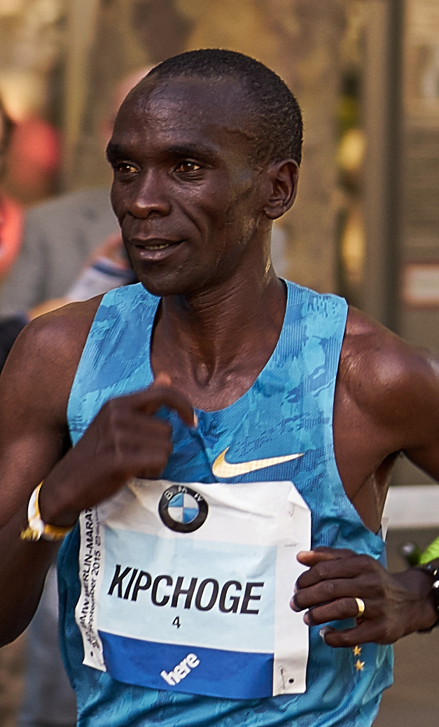
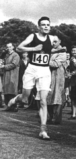
Alan Turing

|
|
Probability Winning Olympics?
- He was a formidable Marathon runner.
- In 1946 he ran a time 2 hours 46 minutes.
- That’s a pace of 3.95 min/km.
- What is the probability he would have won an Olympics if one had been held in 1946?
Running Example: Olympic Marathons
Maximum Likelihood: Iterative Solution
\[ E(m, c) = \sum_{i=1}^n(y_i-mx_i-c)^2 \]
Coordinate Descent
Learning is Optimisation
- Learning is minimisation of the cost function.
- At the minima the gradient is zero.
- Coordinate descent, find gradient in each coordinate and set to zero. \[\frac{\text{d}E(c)}{\text{d}c} = -2\sum_{i=1}^n\left(y_i- m x_i - c \right)\] \[0 = -2\sum_{i=1}^n\left(y_i- mx_i - c \right)\]
Learning is Optimisation
- Fixed point equations \[0 = -2\sum_{i=1}^ny_i +2\sum_{i=1}^nm x_i +2n c\] \[c = \frac{\sum_{i=1}^n\left(y_i - mx_i\right)}{n}\]
Learning is Optimisation
- Learning is minimisation of the cost function.
- At the minima the gradient is zero.
- Coordinate descent, find gradient in each coordinate and set to zero. \[\frac{\text{d}E(m)}{\text{d}m} = -2\sum_{i=1}^nx_i\left(y_i- m x_i - c \right)\] \[0 = -2\sum_{i=1}^nx_i \left(y_i-m x_i - c \right)\]
Learning is Optimisation
- Fixed point equations \[0 = -2\sum_{i=1}^nx_iy_i+2\sum_{i=1}^nm x_i^2+2\sum_{i=1}^ncx_i\] \[m = \frac{\sum_{i=1}^n\left(y_i -c\right)x_i}{\sum_{i=1}^nx_i^2}\]
\[m^* = \frac{\sum_{i=1}^n(y_i - c)x_i}{\sum_{i=1}^nx_i^2}\]
Fixed Point Updates
\[ \begin{aligned} c^{*}=&\frac{\sum _{i=1}^{n}\left(y_i-m^{*}x_i\right)}{n},\\ m^{*}=&\frac{\sum _{i=1}^{n}x_i\left(y_i-c^{*}\right)}{\sum _{i=1}^{n}x_i^{2}},\\ \left.\sigma^2\right.^{*}=&\frac{\sum _{i=1}^{n}\left(y_i-m^{*}x_i-c^{*}\right)^{2}}{n} \end{aligned} \]
Coordiate Descent Algorithm
Contour Plot of Error Function
Regression Coordiate Fit
Important Concepts Not Covered
- Other optimization methods:
- Second order methods, conjugate gradient, quasi-Newton and Newton.
- Effective heuristics such as momentum.
- Local vs global solutions.
Multivariate Regression
Multi-dimensional Inputs
- Multivariate functions involve more than one input.
- Height might be a function of weight and gender.
- There could be other contributory factors.
- Place these factors in a feature vector \(\mathbf{ x}_i\).
- Linear function is now defined as \[f(\mathbf{ x}_i) = \sum_{j=1}^p w_j x_{i, j} + c\]
Vector Notation
- Write in vector notation, \[f(\mathbf{ x}_i) = \mathbf{ w}^\top \mathbf{ x}_i + c\]
- Can absorb \(c\) into \(\mathbf{ w}\) by assuming extra input \(x_0\) which is always 1. \[f(\mathbf{ x}_i) = \mathbf{ w}^\top \mathbf{ x}_i\]
Log Likelihood for Multivariate Regression
The likelihood of a single data point is
\[p\left(y_i|x_i\right)=\frac{1}{\sqrt{2\pi\sigma^2}}\exp\left(-\frac{\left(y_i-\mathbf{ w}^{\top}\mathbf{ x}_i\right)^{2}}{2\sigma^2}\right).\]
Log Likelihood for Multivariate Regression
Leading to a log likelihood for the data set of
Error Function
And a corresponding error function of \[E(\mathbf{ w},\sigma^2)=\frac{n}{2}\log\sigma^2 + \frac{\sum_{i=1}^{n}\left(y_i-\mathbf{ w}^{\top}\mathbf{ x}_i\right)^{2}}{2\sigma^2}.\]
Quadratic Loss
\[ E(\mathbf{ w}) = \sum_{i=1}^n\left(y_i - f(\mathbf{ x}_i, \mathbf{ w})\right)^2 \]
Linear Model
\[ E(\mathbf{ w}) = \sum_{i=1}^n\left(y_i - \mathbf{ w}^\top \mathbf{ x}_i\right)^2 \]
Bracket Expansion
\[ \begin{align*} E(\mathbf{ w},\sigma^2) = & \frac{n}{2}\log \sigma^2 + \frac{1}{2\sigma^2}\sum _{i=1}^{n}y_i^{2}-\frac{1}{\sigma^2}\sum _{i=1}^{n}y_i\mathbf{ w}^{\top}\mathbf{ x}_i\\&+\frac{1}{2\sigma^2}\sum _{i=1}^{n}\mathbf{ w}^{\top}\mathbf{ x}_i\mathbf{ x}_i^{\top}\mathbf{ w} +\text{const}.\\ = & \frac{n}{2}\log \sigma^2 + \frac{1}{2\sigma^2}\sum _{i=1}^{n}y_i^{2}-\frac{1}{\sigma^2} \mathbf{ w}^\top\sum_{i=1}^{n}\mathbf{ x}_iy_i\\&+\frac{1}{2\sigma^2} \mathbf{ w}^{\top}\left[\sum _{i=1}^{n}\mathbf{ x}_i\mathbf{ x}_i^{\top}\right]\mathbf{ w}+\text{const}. \end{align*} \]
Design Matrix
\[ \mathbf{X} = \begin{bmatrix} \mathbf{ x}_1^\top \\\ \mathbf{ x}_2^\top \\\ \vdots \\\ \mathbf{ x}_n^\top \end{bmatrix} = \begin{bmatrix} 1 & x_1 \\\ 1 & x_2 \\\ \vdots & \vdots \\\ 1 & x_n \end{bmatrix} \]
Writing the Objective with Linear Algebra
\[ E(\mathbf{ w}) = \sum_{i=1}^n(y_i - f(\mathbf{ x}_i; \mathbf{ w}))^2, \]
\[ f(\mathbf{ x}_i; \mathbf{ w}) = \mathbf{ x}_i^\top \mathbf{ w}. \]
Stacking Vectors
\[ \mathbf{ f}= \begin{bmatrix}f_1\\f_2\\ \vdots \\ f_n\end{bmatrix}. \]
\[ E(\mathbf{ w}) = (\mathbf{ y}- \mathbf{ f})^\top(\mathbf{ y}- \mathbf{ f}) \]
\[ \mathbf{ f}= \mathbf{X}\mathbf{ w}. \]
\[ E(\mathbf{ w}) = (\mathbf{ y}- \mathbf{ f})^\top(\mathbf{ y}- \mathbf{ f}) \]
Objective Optimization
Multivariate Derivatives
- We will need some multivariate calculus.
- For now some simple multivariate differentiation: \[\frac{\text{d}{\mathbf{a}^{\top}}{\mathbf{ w}}}{\text{d}\mathbf{ w}}=\mathbf{a}\] and \[\frac{\mathbf{ w}^{\top}\mathbf{A}\mathbf{ w}}{\text{d}\mathbf{ w}}=\left(\mathbf{A}+\mathbf{A}^{\top}\right)\mathbf{ w}\] or if \(\mathbf{A}\) is symmetric (i.e. \(\mathbf{A}=\mathbf{A}^{\top}\)) \[\frac{\text{d}\mathbf{ w}^{\top}\mathbf{A}\mathbf{ w}}{\text{d}\mathbf{ w}}=2\mathbf{A}\mathbf{ w}.\]
Differentiate the Objective
\[ \frac{\partial L\left(\mathbf{ w},\sigma^2 \right)}{\partial \mathbf{ w}}=\frac{1}{\sigma^2} \sum _{i=1}^{n}\mathbf{ x}_i y_i-\frac{1}{\sigma^2} \left[\sum _{i=1}^{n}\mathbf{ x}_i\mathbf{ x}_i^{\top}\right]\mathbf{ w} \] Leading to \[ \mathbf{ w}^{*}=\left[\sum _{i=1}^{n}\mathbf{ x}_i\mathbf{ x}_i^{\top}\right]^{-1}\sum _{i=1}^{n}\mathbf{ x}_iy_i, \]
Differentiate the Objective
Rewrite in matrix notation: \[ \sum_{i=1}^{n}\mathbf{ x}_i\mathbf{ x}_i^\top = \mathbf{X}^\top \mathbf{X} \] \[ \sum_{i=1}^{n}\mathbf{ x}_iy_i = \mathbf{X}^\top \mathbf{ y} \]
Update Equation for Global Optimum
Update Equations
Solve the matrix equation for \(\mathbf{ w}\). \[\mathbf{X}^\top \mathbf{X}\mathbf{ w}= \mathbf{X}^\top \mathbf{ y}\]
The equation for \(\left.\sigma^2\right.^{*}\) may also be found \[\left.\sigma^2\right.^{{*}}=\frac{\sum_{i=1}^{n}\left(y_i-\left.\mathbf{ w}^{*}\right.^{\top}\mathbf{ x}_i\right)^{2}}{n}.\]
Movie Violence Data
- Data containing movie information (year, length, rating, genre, IMDB Rating).
- Try and predict what factors influence a movie’s violence
Multivariate Regression on Movie Violence Data
- Regress from features
Year,Body_Count,Length_MinutestoIMDB_Rating.
Residuals
Solution with QR Decomposition
\[ \mathbf{X}^\top \mathbf{X}\boldsymbol{\beta} = \mathbf{X}^\top \mathbf{ y} \] substitute \(\mathbf{X}= \mathbf{Q}\mathbf{R}\) \[ (\mathbf{Q}\mathbf{R})^\top (\mathbf{Q}\mathbf{R})\boldsymbol{\beta} = (\mathbf{Q}\mathbf{R})^\top \mathbf{ y} \] \[ \mathbf{R}^\top (\mathbf{Q}^\top \mathbf{Q}) \mathbf{R} \boldsymbol{\beta} = \mathbf{R}^\top \mathbf{Q}^\top \mathbf{ y} \]
\[ \mathbf{R}^\top \mathbf{R} \boldsymbol{\beta} = \mathbf{R}^\top \mathbf{Q}^\top \mathbf{ y} \] \[ \mathbf{R} \boldsymbol{\beta} = \mathbf{Q}^\top \mathbf{ y} \]
- More nummerically stable.
- Avoids the intermediate computation of \(\mathbf{X}^\top\mathbf{X}\).
Thanks!
- company: Trent AI
- book: The Atomic Human
- twitter: @lawrennd
- The Atomic Human
- newspaper: Guardian Profile Page
- blog: http://inverseprobability.com
Further Reading
For fitting linear models: Section 1.1-1.2 of Rogers and Girolami (2011)
Section 1.2.5 up to equation 1.65 of Bishop (2006)
Section 1.3 for Matrix & Vector Review of Rogers and Girolami (2011)