

Week 5: Maximum Entropy and the Exponential Family
[jupyter][google colab][reveal][edit]
Abstract:
Jaynes’ maximum entropy principle, the exponential family as the MaxEnt family, and the first synthesis of the three operational readings of entropy. This is the intended answer to “how is entropy understood today?” to be revised again after von Neumann entropy in week 8.
Worksheet 2 is due at the start of this session. Quiz 2 occupies the first ten minutes (MaxEnt, exponential family, Landauer).
This Session
Time plan (120 minutes)
| Minutes | Block |
|---|---|
| 0–10 | Quiz 2 (Moodle); collect Worksheet 2 |
| 10–55 | Laplace \(\to\) Jaynes; Lagrange; die and Gaussian |
| 55–65 | Break |
| 65–85 | MaxEnt proof \(\to\) exponential family; \(\theta=-\lambda\) |
| 85–100 | Examples: Bernoulli, softmax, two-spin |
| 100–110 | Legendre transform: \(F=U-TS\) again; \(H=A-\theta\cdot\eta\) |
| 110–120 | LO7 synthesis; “how is entropy understood today?” |
Information, energy and intelligence course notebook setup
We install some bespoke code for creating and saving plots as well as loading data sets.
import importlib.utilcmd = install_command('pods')%system {cmd}cmd = install_command('notutils')%system {cmd}cmd = install_command('mlai')%system {cmd}Maximum Entropy
Lagrange Multipliers
Many problems in physics, engineering and machine learning ask us to optimise a function subject to constraints. For example, we free energy minimisation, or maximising entropy while matching observed averages.1 Principal component analysis can be formulated as finding directions in data of maximum variance. Each direction is constrained to be orthogonal to the previous one. Lagrange multipliers turn these constrained problems into unconstrained ones.
One Equality Constraint
If we want to find a stationary point of a function, \(f(\mathbf{x})\), and we know that another function \(g(\mathbf{x}) = c\) is constrained such that \(g(\mathbf{x}) = c\) we introduce a Lagrange multiplier, often denoted by \(\lambda\) and form the Lagrangian, \[ \mathscr{L}(\mathbf{x}, \lambda) = f(\mathbf{x}) + \lambda\bigl(g(\mathbf{x}) - c\bigr). \] We are optimising with respect to \(\mathbf{x}\) and the gradient of the Lagrangian is given by \[ \nabla_{\mathbf{x}} \mathscr{L} = \nabla f + \lambda \nabla g, \] but we now also have the gradient of the Lagrangian with respect to the Lagrange multiplier, \[ \frac{\partial \mathscr{L}}{\partial \lambda} = g(\mathbf{x}) - c. \] Think about what happens when we set both gradients to zero (as we would do if we were looking for a stationary point of an unconstrained function). The first equation is now \[ \nabla f + \lambda \nabla g = \mathbf{0} \] which tells us that \(\nabla f\) is parallel to \(\nabla g\), and therefore the gradient of the objective, \(\nabla f\), is perpendicular to the constraint surface.
Figure: At stationarity, \(\nabla f + \lambda\nabla g = \mathbf{0}\): the objective gradient is balanced by the constraint gradient scaled by \(\lambda\) (here \(\lambda = -\frac{1}{2}\) in the worked example).
The second condition, \[ g(\mathbf{x}) - c = 0, \] just enforces the constraint itself (\(g(\mathbf{x}) = c\)).
Picture climbing a hill (maximise \(f\)) while staying on a path defined by \(g(\mathbf{x}) = c\). At the highest point reachable on the path, you cannot move along the path and still increase \(f\). That means \(\nabla f\) points off the path, normal to the constraint surface. The multiplier \(\lambda\) measures how strongly the constraint must pull against the unconstrained gradient.
Several Equality Constraints
With multiple constraints \(g_k(\mathbf{x}) = c_k\) for \(k = 1, \ldots, m\), introduce one multiplier \(\lambda_k\) for each constraint: \[ \mathscr{L}(\mathbf{x}, \boldsymbol{\lambda}) = f(\mathbf{x}) + \sum_{k=1}^m \lambda_k \bigl(g_k(\mathbf{x}) - c_k\bigr). \] Stationarity gives \[\begin{align} \nabla f + \sum_{k=1}^m \lambda_k \nabla g_k &= 0, \\ g_k(\mathbf{x}) &= c_k \quad k = 1, \ldots, m. \end{align}\] Each multiplier enforces one constraint; together they specify how far the objective gradient is rotated onto the intersection of the constraint surfaces.
A Worked Example
The method is clearer on a small problem before we apply it to probabilities. Minimise \[ f(x,y) = \frac{1}{2}(x^2 + y^2) \] subject to the linear constraint \(x + y = 1\). Geometrically, we seek the point on the line closest to the origin; physically, this is the same pattern as minimising a quadratic energy or loss while a conserved quantity remains fixed. The Lagrangian is \[ \mathscr{L}(x,y,\lambda) = \frac{1}{2}(x^2 + y^2) + \lambda(x + y - 1). \] Stationarity gives \(x + \lambda = 0\), \(y + \lambda = 0\), and \(x + y = 1\), hence \(x = y = \frac{1}{2}\) and \(\lambda = -\frac{1}{2}\). The gradient of \(f\) at the solution is \((1,1)\), parallel to the constraint normal \((1,1)\) as required.
The same template appears in machine learning: minimise a squared error or regulariser \(\frac{1}{2}\|\mathbf{w}\|^2\) subject to a linear prediction constraint \(\mathbf{w}^\top \mathbf{x} = y\). The multiplier \(\lambda\) then plays the role of a Lagrange multiplier in ridge regression and support-vector margins. We do not need that full story here; the point is that one constraint adds one multiplier and reduces the problem to solving linear stationarity conditions.
Principle of Insufficient Reason
Pierre-Simon Laplace
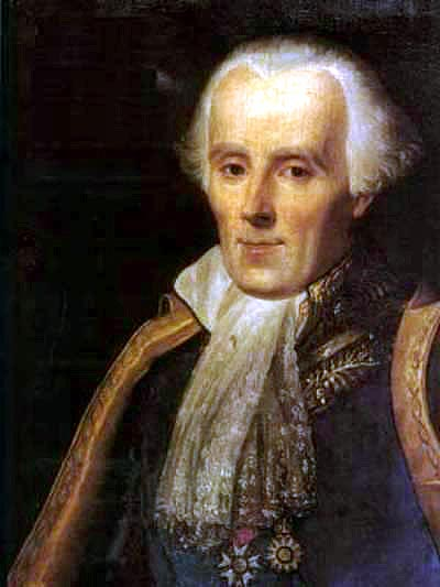
Figure: Pierre-Simon Laplace 1749-1827.
From Laplace’s perspective we use probability to deal with our ignorance about the data, the physical lawas and the computation. This is Laplace’s gremlin. But how do we estimate probabilities? How do we assign \(p\) when we know almost nothing?
Laplace’s principle of insufficient reason suggestd that if we have mutually exclusive outcomes and nothing distinguishes one from the other then we should asign them equal probability, i.e. \(p_i = \tfrac{1}{n}\).
The Philosophical Essay on Probabilities (Laplace, 1814) argued that probability is relative in part to our ignorance and in part to our knowledge. So when we know that only one of \(n\) mutually exclusive and exhaustive outcomes must occur we don’t have any reason to prefer one over the other. This suggests that we should assign \[\begin{align} p_i = \frac{1}{n}, \qquad i = 1,\ldots,n. \end{align}\] This known as Laplace’s principle of insufficient reason or the principle of indifference. It’s an assignment athat is ‘least-commital’ but consistent with the information we have. In this case the information we have is the different possibilities (the \(n\) outcomes) and the need for normalisation.
Example: Will the sun rise tomorrow?
As an example Laplace considered what the probability that the sun rises tomorrow is. To our knowledge, the sun has risen every day. So is the probability 100%? The example comes from Philosophical Essay on Probabilities (Laplace, 1814).
Figure: Each update is belief \(\times\) likelihood \(\rightarrow\) posterior; a reset frame then promotes the posterior to the new prior (likelihood cleared). Early steps use one more sunrise (\(\propto\theta\)); the jump to \(n=20\) uses the likelihood for \(17\) further rises (\(\propto\theta^{17}\)).
The animation peels probability mass toward \(\theta=1\). Quantify that with the differential entropy of the belief, \[\begin{align} H[p] = -\int_0^1 p(\theta)\log p(\theta)\,\mathrm{d}\theta. \end{align}\] Under insufficient reason the prior is uniform on \([0,1]\), so \(p(\theta)=1\) and \[\begin{align} H_0 = -\int_0^1 1\cdot\log 1\,\mathrm{d}\theta = 0. \end{align}\] After \(n\) sunrises the normalised belief is \(p_n(\theta)=(n+1)\theta^{n}\). Substitute and use \(\int_0^1\theta^{n}\,\mathrm{d}\theta=1/(n+1)\) together with \(\int_0^1\theta^{n}\log\theta\,\mathrm{d}\theta=-1/(n+1)^2\): \[\begin{align} H_n &= -\int_0^1 (n+1)\theta^{n}\bigl(\log(n+1)+n\log\theta\bigr)\,\mathrm{d}\theta = \frac{n}{n+1}-\log(n+1). \end{align}\] Each sunrise reduces this entropy (the number becomes more negative as the density sharpens). The information gained on day \(n\) is the drop \[\begin{align} I_n = H_{n-1}-H_n = \log\!\left(1+\frac{1}{n}\right)-\frac{1}{n(n+1)}. \end{align}\] The first day buys \(I_1=\log 2-\tfrac12\approx 0.193\) nats; the second buys slightly more (\(I_2\approx 0.239\)); thereafter \(I_n\) falls, asymptotically like \(1/(2n^2)\). After Laplace’s \(n\approx 1.8\times 10^6\) days, \(H_n\approx 1-\log n\) is large and negative, and each further day adds almost no information about \(\theta\).
Figure: Differential entropy \(H_n\) of \(p(\theta)\) after \(n\) sunrises, and the information \(I_n\) gained on day \(n\). The prior sits at \(H_0=0\); each success drives \(H_n\) downward.
A second, coarser reading is the binary entropy of tomorrow’s predictive probability \(p_n=(n+1)/(n+2)\): \[\begin{align} h(p_n)=-p_n\log p_n-(1-p_n)\log(1-p_n), \end{align}\] which starts at \(h(1/2)=\log 2\) and falls toward \(0\) as \(p_n\to 1\). That tracks uncertainty about the next day, whereas \(H_n\) tracks uncertainty about the latent rate \(\theta\).
Laplace applies insufficient reason not only to discrete outcomes, but to an unknown daily rate \(\theta\in[0,1]\). Knowing nothing about \(\theta\), he places a uniform prior \(p(\theta)=1\) on the unit interval. Every recorded day is a success: the sun rose. After \(n\) independent rises the likelihood is \(\theta^n\), so \[\begin{align} p(\theta\mid n\text{ rises}) \propto \theta^{n}, \end{align}\] and the probability of one further rise is the posterior mean \[\begin{align} P(\text{rises tomorrow}\mid n\text{ rises}) = \int_0^1 \theta\, p(\theta\mid n\text{ rises})\,\mathrm{d}\theta = \frac{n+1}{n+2}. \end{align}\] This is Laplace’s rule of succession (the same “\(+1\), \(+2\)” that later appears as Laplace smoothing). In modern notation the posterior is \(\mathrm{Beta}(n+1,1)\); after each new sunrise it becomes \(\mathrm{Beta}(n+2,1)\), more sharply peaked at \(\theta=1\), while the predictive odds move from \(1{:}1\) toward certainty without ever quite reaching it.
Laplace did not have the Beta distribution by name, and he did not need the Laplace approximation for this result. In the 1774 memoir on inverse probability he evaluates the normalising integrals exactly — what we now write as \(\int_0^1 \theta^{n}\,\mathrm{d}\theta = 1/(n+1)\) — via what he called Euler’s series. The Beta language is modern packaging of that calculation. The Laplace approximation (a local Gaussian expansion of an integrand about its mode) is a different tool, also named after him; it is not how the rule of succession was obtained.
In the Essay he takes the oldest historical epoch as five thousand years, or \(n=1{,}826{,}213\) days of recorded sunrise, and concludes that — on this information alone — the odds on tomorrow’s sunrise are \(1{,}826{,}214\) to one. He then adds, in the next sentence, that for anyone who recognises the astronomical regularity of days and seasons the probability is incomparably greater. The sunrise calculation is a demonstration of the rule under deliberate ignorance of mechanism, not Laplace’s estimate of whether the sun will rise.
So the preliminary example already shows the pattern we need: insufficient reason supplies the prior of ignorance; each success updates it and peels a little more mass away from small \(\theta\); the predictive probability is not the raw frequency \(n/n=1\).
The principle of insufficient reason, and the rule of succession built from it, answer the case where our information is a list of possibilities and (optionally) raw counts. As soon as we know more — a mean face value on a die, a mean energy, a variance — equal weights, or a uniform prior on a single rate, may fail to encode that information. Jaynes’ maximum entropy principle extends Laplace’s idea: among all distributions that match the stated constraints, choose the one that maximises Shannon entropy \(H(p)=-\sum_i p_i\log p_i\). That choice is maximally noncommittal with respect to everything else.
With only the normalisation constraint \(\sum_i p_i=1\), MaxEnt recovers Laplace’s uniform assignment \(p_i=1/n\). With an additional mean-energy constraint, the same calculation yields Boltzmann weights. With mean and variance, it yields a Gaussian. The exponential family is therefore the family of distributions that generalise insufficient reason from “we know nothing” (or “we know only these counts”) to “we know these moments and nothing more.”
Critiques of bare indifference (Bertrand’s paradox and related reparameterisation puzzles) motivate the need for an explicit state space and explicit constraints — which is exactly what the MaxEnt formalism supplies. We will not pursue those paradoxes here; the operational fix is to state what is held fixed before maximising \(H\). Laplace’s own sunrise caveat makes the same point in plain language: once you know the mechanism, you no longer pretend to know only the counts.
Jaynes and Maximum Entropy
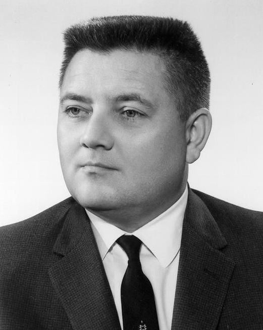
Figure: Ed Jaynes who developed the maximum entropy principle
Maximum Entropy Motivation
Ed Jaynes (Jaynes, 1957), proposed a foundation for statistical mechanics based on information theory. Jaynes recast that the problem of assigning probabilities in statistical mechanics as a problem of inference with incomplete information.
A central problem in statistical mechanics is assigning initial probabilities when our knowledge is incomplete. The canonical example is if we know only the average energy of a system, what probability distribution should we use? Jaynes argued that we should use the distribution that maximises entropy subject to the constraints of our knowledge.
Jaynes illustrated the approach with a simple example. If a die has been tossed many times, with an average result of 4.5 rather than the expected 3.5 for a fair die. What probability assignment \(P_n\) (\(n=1,2,...,6\)) should we make for the next toss?
We need to satisfy two constraints \[\begin{align} \sum_{n=1}^6 P_n &= 1 \\ \sum_{n=1}^6 n P_n &= 4.5 \end{align}\]
Many distributions could satisfy these constraints, but which one makes the fewest unwarranted assumptions? Jaynes argued that we should choose the distribution that is maximally noncommittal with respect to missing information - the one that maximises the entropy, \[\begin{align} S_I = -\sum_{i} p_i \log p_i \end{align}\] This principle leads to the exponential family of distributions, which in statistical mechanics gives us the canonical ensemble and other familiar distributions.
Die Roll Simulation
This simulation illustrates the maximum entropy principle through Jaynes’ dice example (Jaynes, 1957). A fair die has expected outcome 3.5; the Jaynes example asks: if we know only that the average outcome is 4.5, what probability distribution \(P_n\) over the six faces should we assign?
The answer is the maximum-entropy distribution subject to the constraint \(\sum_{n=1}^6 n P_n = 4.5\), which belongs to the exponential family: \[\begin{align} P_n = \frac{e^{\lambda n}}{Z(\lambda)}, \qquad Z(\lambda) = \sum_{n=1}^6 e^{\lambda n} \end{align}\] where \(\lambda > 0\) is chosen so the mean constraint is satisfied. This avoids any unwarranted assumption beyond the available data.
Rolls: 0
Sample mean: —
H(p): —
Outcome weights (auto-normalised to probabilities)
Figure: Interactive die-roll simulation. Click the die or press Roll to sample from the configured distribution. The histogram shows empirical relative frequencies (coloured bars) overlaid on the theoretical probabilities (dashed outlines). Use the sliders to set arbitrary outcome weights, or click a preset to load the uniform distribution (mean 3.5), the Jaynes maximum-entropy distribution (mean 4.5), the simple 50/50 distribution (faces 4 and 5 equally, mean 4.5 with minimal entropy), or a low-biased distribution (mean 2).
Maximum entropy is the week’s pair in one move: entropy forbids assuming more structure than the constraints; probability is the recipe. One mean-energy constraint gives Boltzmann weights; mean and variance give the Gaussian. The Lagrange multiplier on energy is coldness \(\beta\).
Figure: Jaynes’ die: MaxEnt subject to mean 4.5 versus the uniform distribution.
Derivation of the Boltzmann Distribution
For a given mean energy \(U\), among all distributions with that \(U\), pick the one with largest entropy. Week 2 named the Gibbs–Boltzmann occupation; this is the MaxEnt derivation that earns it.
Maximum entropy subject to normalisation and fixed mean energy gives \(p_i = e^{-\beta E_i}/Z\). The Lagrange multiplier on the energy constraint is coldness \(\beta\) from weeks 1–2.
Figure: Occupation of a two-state system as coldness increases. At low \(\beta\) both states are populated; at high \(\beta\) the ground state dominates.
# Live check: boltzmann([0, 1], 1.0) -> (0.731, 0.269)
boltzmann([0, 1], 1.0)
MaxEnt Under Constraints: the Proof
Fix a finite outcome set \(\{x_1,\ldots,x_n\}\) and unknown probabilities \(p_i>0\). The maximum entropy principle asks for the \(p_i\) that maximise Shannon entropy \[\begin{align} H(p) = -\sum_{i=1}^n p_i \log p_i \end{align}\] subject to normalisation and \(m\) moment constraints \[\begin{align} \sum_{i=1}^n p_i = 1, \qquad \sum_{i=1}^n p_i f_k(x_i) = \langle f_k\rangle \quad (k=1,\ldots,m). \end{align}\] Introduce Lagrange multipliers \(\lambda_0,\lambda_1,\ldots,\lambda_m\) and form \[\begin{align} \mathscr{L}(p,\lambda) = \sum_i p_i \log p_i + \lambda_0\Bigl(\sum_i p_i - 1\Bigr) + \sum_{k=1}^m \lambda_k\Bigl(\sum_i p_i f_k(x_i) - \langle f_k\rangle\Bigr). \end{align}\] At an interior maximum, \(\partial \mathscr{L}/\partial p_i = 0\) gives \[\begin{align} \log p_i + 1 + \lambda_0 + \sum_{k=1}^m \lambda_k f_k(x_i) = 0, \end{align}\] so \[\begin{align} p_i = \exp\Bigl(-1-\lambda_0\Bigr)\, \exp\Bigl(-\sum_{k=1}^m \lambda_k f_k(x_i)\Bigr). \end{align}\] Absorbing \(\exp(-1-\lambda_0)\) into the normalisation constant, \[\begin{align} p_i = \frac{\exp\bigl(-\sum_{k=1}^m \lambda_k f_k(x_i)\bigr)} {Z(\lambda_1,\ldots,\lambda_m)}, \qquad Z = \sum_{i=1}^n \exp\Bigl(-\sum_{k=1}^m \lambda_k f_k(x_i)\Bigr). \end{align}\] The multipliers are fixed by substituting this \(p\) back into the constraints. The maximum entropy is \[\begin{align} H_{\max} = \log Z + \sum_{k=1}^m \lambda_k \langle f_k\rangle. \end{align}\] This is the same calculation as Jaynes’ die (one linear constraint on the face value) and, with \(f_1(x_i)=E_i\), the canonical ensemble.
The constrained MaxEnt distribution is not merely like an exponential family — on a finite (or countable) state space it is one. Take sufficient statistics \(T_k(x)=f_k(x)\). Then the MaxEnt assignment is \[\begin{align} p(x\mid\boldsymbol{\theta}) = \exp\bigl(\boldsymbol{\theta}\cdot T(x) - A(\boldsymbol{\theta})\bigr)\, h(x), \end{align}\] with \(h(x)\) the counting measure on the allowed outcomes and \[\begin{align} A(\boldsymbol{\theta}) = \log \sum_x \exp\bigl(\boldsymbol{\theta}\cdot T(x)\bigr). \end{align}\] The Lagrange multipliers from the proof are the negative natural parameters: \[\begin{align} \theta_k = -\lambda_k. \end{align}\] We use the minus sign so that high-energy states are down-weighted when \(\theta_1=-\beta<0\) in the canonical ensemble. The constraint values enter through the Legendre dual: \(\eta_k = \langle T_k\rangle = \partial A/\partial \theta_k\), and the \(\lambda_k\) (equivalently \(\theta_k\)) are chosen so these expectations match the data. Weeks 6–7 reuse this pair \((\boldsymbol{\theta},\boldsymbol{\eta})\) as dual coordinates on the same manifold.
Continuous \(x\) is the same pattern with sums replaced by integrals; Gaussian MaxEnt (mean and variance fixed) is the flagship continuous example. Softmax and the two-spin Hamiltonian later in this lecture are the same theorem with richer \(T(x)\).
The General Maximum-Entropy Formalism
For a more general case, suppose a quantity \(x\) can take values \((x_1, x_2, \ldots, x_n)\) and we know the average values of several functions \(f_k(x)\). The problem is to find the probability assignment \(p_i = p(x_i)\) that satisfies \[\begin{align} \sum_{i=1}^n p_i &= 1 \\ \sum_{i=1}^n p_i f_k(x_i) &= \langle f_k(x) \rangle = F_k \quad k=1,2,\ldots,m \end{align}\] and maximises the entropy \(S_I = -\sum_{i=1}^n p_i \log p_i\).
Using Lagrange multipliers, the solution is the generalised canonical distribution, \[\begin{align} p_i = \frac{\exp(-\lambda_1 f_1(x_i) - \ldots - \lambda_m f_m(x_i))}{Z(\lambda_1,\ldots,\lambda_m)} \end{align}\] where \(Z(\lambda_1,\ldots,\lambda_m)\) is the partition function, \[\begin{align} Z(\lambda_1,\ldots,\lambda_m) = \sum_{i=1}^n \exp(-\lambda_1 f_1(x_i) - \ldots - \lambda_m f_m(x_i)) \end{align}\] The Lagrange multipliers \(\lambda_k\) are determined by the constraints, \[\begin{align} \langle f_k \rangle = -\frac{\partial}{\partial \lambda_k}\log Z(\lambda_1,\ldots,\lambda_m) \quad k=1,2,\ldots,m. \end{align}\] The maximum attainable entropy is \[\begin{align} (S_I)_{max} = \log Z + \sum_{k=1}^m \lambda_k \langle f_k \rangle. \end{align}\]
\[ p_i = \frac{\exp(-\lambda_1 f_1(x_i) - \ldots - \lambda_m f_m(x_i))}{Z(\lambda_1,\ldots,\lambda_m)} \] \[ Z(\ldots) = \sum_{i=1}^n \exp(-\lambda_1 f_1(x_i) - \ldots - \lambda_m f_m(x_i)) \] \[ \langle f_k \rangle = -\frac{\partial}{\partial \lambda_k}\log Z(\lambda_1,\ldots,\lambda_m) \quad k=1,2,\ldots,m. \]
The Exponential Family
Exponential Families
The exponential family is a class of probability distributions that plays a central role in information theory and statistical mechanics. For our purposes, these distributions have particularly elegant properties when we work with their natural parameters.
Definition
A probability distribution belongs to the exponential family if it can be written in the form \[
p(\mathbf{x} | \boldsymbol{\theta}) = \exp\left(\boldsymbol{\theta}^\top T(\mathbf{x}) - \mathcal{A}(\boldsymbol{\theta})\right) h(\mathbf{x}),
\] where - \(\boldsymbol{\theta} \in \mathbb{R}^d\) are the natural parameters - \(T(\mathbf{x})\) are the sufficient statistics
- \(\mathcal{A}(\boldsymbol{\theta})\) is the log partition function (ensures normalization) - \(h(\mathbf{x})\) is the base measure (often constant)
The natural parameters are called “natural” because they appear linearly in the exponent. This parametrization has special geometric properties that make information-theoretic calculations particularly clean. As we’ll see, working with these connections makes the connections between probability theory and geometry particularly clean.
The Log Partition Function as Cumulant Generator
The setup of the exponential family ensures that the log partition function operates as a cumulant generating function. We denote it by \(\mathcal{A}(\boldsymbol{\theta})\) and it ensures the distribution is normalised. \[ \mathcal{A}(\boldsymbol{\theta}) = \log \int \exp\left(\boldsymbol{\theta}^\top T(\mathbf{x})\right) h(\mathbf{x}) \, d\mathbf{x}. \] But \(\mathcal{A}\)’s role as cumulant generating function also means that we can compute the distributions cumulants through taking its derivatives.
\[ \mathcal{A}(\boldsymbol{\theta}) = \log \int \exp\left(\boldsymbol{\theta}^\top T(\mathbf{x})\right) h(\mathbf{x}) \, d\mathbf{x} \]}
The derivatives of \(\mathcal{A}\) with respect to \(\boldsymbol{\theta}\) give us the cumulants as follows. - First derivative (first cumulant): \(\nabla \mathcal{A}(\boldsymbol{\theta}) = \mathbb{E}[T(\mathbf{x})]\) (the mean) - Second derivative (second cumulant): \(\nabla^2 \mathcal{A}(\boldsymbol{\theta}) = \mathrm{Cov}[T(\mathbf{x})]\) (the covariance) - Higher derivatives: Third and higher cumulants (skewness, kurtosis, etc.)
Connection to Fisher Information
For an exponential family, the second derivative of the log partition function has a special meaning. It is the Fisher information matrix: \[ G(\boldsymbol{\theta}) = \nabla^2 \mathcal{A}(\boldsymbol{\theta}) = \mathrm{Cov}_{\boldsymbol{\theta}}[T(\mathbf{x})]. \] R.A. Fisher introduced this quantity in the context of statistical estimation. Through the Cramér-Rao bound, Fisher information tells us how accurately we can estimate parameters from data, higher Fisher information means better estimation is possible.
The Fisher information is both the Hessian of the log partition function and the covariance of the sufficient statistics. This dual role arises from the log partition function being the cumulant generating function. As we’ll see in the next section, the Fisher information matrix also defines the geometry of the information space.
Entropy in Natural Coordinates
The joint entropy of an exponential family distribution has a straightforward form in natural coordinates, \[ H(\boldsymbol{\theta}) = -\mathbb{E}_{\boldsymbol{\theta}}[\log p(\mathbf{x}|\boldsymbol{\theta})] = \mathcal{A}(\boldsymbol{\theta}) - \boldsymbol{\theta}^\top \nabla \mathcal{A}(\boldsymbol{\theta}) - \mathbb{E}[\log h(\mathbf{x})]. \] When the base measure \(h(\mathbf{x})\) is constant (or when we measure entropy relative to it), this simplifies to \[ H(\boldsymbol{\theta}) = \mathcal{A}(\boldsymbol{\theta}) - \boldsymbol{\theta}^\top \boldsymbol{\mu}, \] where \(\boldsymbol{\mu} = \nabla \mathcal{A}(\boldsymbol{\theta})\) is the mean of the sufficient statistics.
Now we see the utilty of representing through natural parameers, when we take the gradient of entropy with respect to the natural parameters, many terms cancel, \[ \nabla_{\boldsymbol{\theta}} H = \nabla \mathcal{A}(\boldsymbol{\theta}) - \left(\boldsymbol{\theta}^\top \nabla^2 \mathcal{A} + \nabla \mathcal{A}\right) = -\boldsymbol{\theta}^\top \nabla^2 \mathcal{A} = -G(\boldsymbol{\theta})\boldsymbol{\theta}. \] This simple form for the entropy gradient equals negative Fisher information times natural parameters.
Example: Multivariate Gaussian
Let’s make this concrete with the multivariate Gaussian distribution. A Gaussian with mean \(\boldsymbol{\mu}\) and covariance \(\Sigma\) can be written as: \[ p(\mathbf{x}) = \frac{1}{(2\pi)^{d/2}|\Sigma|^{1/2}} \exp\left(-\frac{1}{2}(\mathbf{x}-\boldsymbol{\mu})^\top\Sigma^{-1}(\mathbf{x}-\boldsymbol{\mu})\right). \] To put this in exponential family form, we need to identify the natural parameters and sufficient statistics.
Gaussian in Exponential Family Form
After expanding the quadratic form and collecting terms, the Gaussian becomes: \[ p(\mathbf{x}) = \exp\left(\boldsymbol{\theta}^\top T(\mathbf{x}) - \mathcal{A}(\boldsymbol{\theta})\right) \cdot \frac{1}{(2\pi)^{d/2}}, \] where: - Natural parameters: \(\boldsymbol{\theta} = \Sigma^{-1}\boldsymbol{\mu}\) (precision-weighted mean) - Sufficient statistics: \(T(\mathbf{x}) = \mathbf{x}\) (the data itself) - Log partition function: \(\mathcal{A}(\boldsymbol{\theta}) = \frac{1}{2}\boldsymbol{\theta}^\top\Sigma\boldsymbol{\theta} + \frac{1}{2}\log|\Sigma|\)
For the Gaussian, we can compute the Fisher information matrix directly: \[ G(\boldsymbol{\theta}) = \nabla^2 \mathcal{A}(\boldsymbol{\theta}) = \Sigma. \] As expected, because the log partition is the covariance matrix. Equivalently, \(G^{-1} = \Sigma^{-1}\) is the precision matrix.
This reveals the intuition behind Fisher’s original concept: - Low variance (high precision) → high Fisher information → parameters easier to estimate (tighter Cramér-Rao bound) - High variance (low precision) → low Fisher information → parameters harder to estimate (looser bound)
Example: Categorical Distribution
Consider a categorical distribution over \(K\) outcomes with probabilities \(\{\pi_1, \ldots, \pi_K\}\) where \(\sum_k \pi_k = 1\). We represent an outcome as a one-hot vector \(\mathbf{x} \in \{0,1\}^K\) where exactly one component is 1.
Categorical in Exponential Family Form
The categorical distribution is: \[ p(\mathbf{x}) = \prod_{k=1}^K \pi_k^{x_k} = \exp\left(\sum_{k=1}^K x_k \log \pi_k\right). \] In exponential family form (using \(K-1\) natural parameters due to the sum-to-one constraint): - Natural parameters: \(\boldsymbol{\theta} = (\log \pi_1, \ldots, \log \pi_{K-1})\) (log probabilities) - Sufficient statistics: \(T(\mathbf{x}) = (x_1, \ldots, x_{K-1})\) (one-hot encoding) - Log partition function: \(\mathcal{A}(\boldsymbol{\theta}) = \log\left(\sum_{k=1}^{K-1} e^{\theta_k} + 1\right)\) (log-sum-exp)
The Fisher information matrix for the categorical distribution is: \[ G_{ij}(\boldsymbol{\theta}) = \begin{cases} \pi_i(1-\pi_i) & \text{if } i=j \\ -\pi_i\pi_j & \text{if } i \neq j \end{cases} \] This matrix encodes how “information” is distributed across categories. When one category dominates (\(\pi_i \approx 1\)), the Fisher information about other categories becomes small—it’s hard to learn about rare events!
Why Exponential Families Matter
Exponential families are not just mathematically convenient, they emerge naturally from underlying principles:
Maximum Entropy: Given constraints on the moments of a distribution, the maximum entropy distribution is in the exponential family (Jaynes, 1957).
Information Geometry: The natural parameters define a coordinate system on the manifold of probability distributions where the Fisher information acts as a Riemannian metric (Amari, 2016).
Sufficient Statistics: The sufficient statistics \(T(\mathbf{x})\) capture all the information in the data needed to estimate \(\boldsymbol{\theta}\), nothing is lost by summarizing data through \(T\).
Computational Tractability: Many operations (computing gradients, conjugate priors, message passing) have closed-form solutions.
For the inaccessible game, exponential families provide the setting where information dynamics have their cleanest mathematical form.
Looking Ahead
We’ll see that the form \(\nabla H = -G(\boldsymbol{\theta})\boldsymbol{\theta}\) is crucial for deriving the dynamics of the inaccessible game. The natural parameters will be our coordinates, the Fisher information will be our “information topography,” and entropy gradients will drive the system’s evolution.
The definition \(p(x\mid\boldsymbol{\theta})=\exp(\boldsymbol{\theta}\cdot T(x)-A(\boldsymbol{\theta}))\) is the notation for what we have just derived. Canonical, Gaussian, and Bernoulli belong because each is MaxEnt for its moments. Softmax is the same calculation with a feature map. The two-spin example is the first sufficient statistic that is a product.
Softmax is MaxEnt with Features
The two-level system from week 1 and the Bernoulli are the same exponential family. Occupancy of the excited state is a bit. The natural parameter is \(\theta = -\beta\varepsilon\) if you are reading a paramagnet, and \(\theta = \log\frac{\pi}{1-\pi}\) if you are reading a coin. The log-partition \(A(\theta)=\log(1+e^{\theta})\) is binary entropy’s conjugate in either language. That is the unary case of LO6, already on the board.
The die constrained the mean of a single coordinate. A classifier constrains the mean of a feature of the pair \((x,y)\). Write \(T(x,y)=f(x,y)\) for a vector of functions you have chosen — a bias, the coordinates of \(x\), an indicator that a word occurs, anything you can compute. MaxEnt subject to \[ \mathbb{E}_{p(y\mid x)\,p_{\mathrm{data}}(x)}[f(x,y)] = \mathbb{E}_{p_{\mathrm{data}}}[f(x,y)] \] is the same Lagrange problem as the die. The solution is \[ p(y\mid x) = \exp\bigl(\theta\cdot f(x,y) - A(\theta;x)\bigr), \] with \(A(\theta;x)=\log\sum_{y'}\exp(\theta\cdot f(x,y'))\) the log-sum-exp over labels. That is softmax. Logistic regression is the two-class case, \(f(x,y)=y\,(1,x)\) for \(y\in\{0,1\}\).
MacKay’s Exercises 22.12–22.13 record the identification: maximum-likelihood fitting of an exponential family matches the moments of \(T\), and MaxEnt with those moments produces the same family (MacKay, 2003). The classifier does not care which story you tell.
Berger et al. (1996) is the natural-language version of this calculation. They constrain binary features of the pair \((x,y)\) — a word in a window, a part of speech, a class — and recover \[ p(y\mid x)=\exp\bigl(\lambda\cdot f(x,y)-A(\lambda;x)\bigr). \] They prove the dual: the MaxEnt distribution in that constrained set is the exponential model of maximum likelihood on the sample. The algorithm is generalized iterative scaling, which is moment matching.
The results are translation decisions in IBM’s Candide system, trained on the Canadian Hansard. For French phrases — stays word-for-word, swaps — a never-swap baseline is 70.2% accurate on 71,555 held-out cases. A MaxEnt model grown to 358 features reaches 80.4%. They also grew models for the French rendering of English and , and for finding rift points at which a French sentence can be split without breaking an alignment.
MacKay then declines to use MaxEnt as a method of inference — the loaded die, he says, is a job for Bayes. Hold that tension for the synthesis. The object on this slide is not in dispute. It is an exponential family whose sufficient statistic is a feature map.
Two Spins, One Coupling
Every MaxEnt example so far constrains a function of one variable: a face, an energy, a bit, a feature of a labelled pair. The next legal constraint is a product. Take two Ising spins \(s_1,s_2\in\{+1,-1\}\) and prescribe the two magnetisations and the correlation, \[\begin{align} \langle s_1\rangle &= m_1, & \langle s_2\rangle &= m_2, & \langle s_1 s_2\rangle &= c. \end{align}\] Four states, three moment constraints, plus normalisation. The sufficient statistic is \(T(s)=(s_1,s_2,s_1 s_2)\). MaxEnt returns the two-spin Ising model (Ising, 1925), \[ p(s_1,s_2) = \exp\bigl(h_1 s_1 + h_2 s_2 + J s_1 s_2 - A(h,J)\bigr). \] The Lagrange multiplier on the correlation is the coupling \(J\). Temperature sits in the multipliers; there is nothing else to introduce.
Physics reads an energy \(H=-(h_1 s_1+h_2 s_2+J s_1 s_2)\) and a Boltzmann occupation. Machine learning reads the smallest Boltzmann machine (Ackley et al., 1985): an undirected pair whose parameters are fit by matching those three moments. Inverse Ising is that fit.
Schneidman et al. (2006) put the same model on retinal spike words. They recorded 40 salamander ganglion cells watching natural movies, binned spikes at 20~ms, and treated each bin as a binary word. Pairwise correlations were weak, but the independent model failed by orders of magnitude: a ten-cell pattern that occurred once a minute was predicted once every three years, and \(P(K=10)\) simultaneous spikes was \(\sim 10^{5}\) times the independent rate. The pairwise MaxEnt model — the Ising model whose \(T\) is the magnetisations and the pairwise products — recovered \(I^{(2)}/I_N\sim 90\%\) of the multi-information in groups of ten cells. That fraction held for different movies, for guinea-pig retina, and for cultured cortex. A stimulus-driven conditional-independence model, with two hundred times as many parameters, did worse. Week 8’s \(I=\sum h_i-H\) is their \(I_N\).
Do not fit a retina today. See that a correlation is a legal \(T\), and that the energy and the classifier are the same exponential family.
Week 7’s \(m\)-projection is this matching, written geometrically. Week 8’s multi-information \(I=\sum h_i-H\) is the extra reduction in joint entropy that \(J\) buys. Paths, caliber, and Schrödinger bridges wait until week 8 (second half). The algorithm that finds the MaxEnt coupling of two prescribed marginals — Sinkhorn, or iterative proportional fitting — waits with them: that is the same exponential family with a different constraint set (the full row and column sums, not three moments). Four states is small enough to write the partition function by hand, \[ Z= e^{J}(e^{h_1+h_2}+e^{-h_1-h_2})+e^{-J}(e^{h_1-h_2}+e^{-h_1+h_2}), \] or to reuse the optimiser from the die.
The Legendre Transform
You have already performed a Legendre transform. In week 2 the Helmholtz free energy \[ F = U - TS \] changed the independent variable from entropy to temperature. The same subtraction, of a product of a conjugate pair, is what relates the log-partition function of an exponential family to its entropy. The object has a name. It is the reason the exponential family has two coordinate charts, and it is why the geometry of weeks 6–7 is dually flat rather than merely Riemannian.
Take a smooth convex function \(\phi(x)\). Its derivative \(y = \phi'(x)\) is a change of coordinate: each slope \(y\) labels a unique point on the graph. The Legendre transform writes the same information as a function of that slope, \[ \phi^*(y) = xy - \phi(x), \] with \(x\) recovered from \(y\) by inversion. Differentiating the conjugate recovers the original coordinate, \(x = (\phi^*)'(y)\). The pair inverts. Nothing is added and nothing is lost. You have changed which quantity you treat as independent.
Internal energy \(U\) is naturally a function of entropy. Temperature is the slope, \(T = \partial U/\partial S\). Helmholtz free energy \[ F(T,V,N) = U - TS \] is the Legendre transform that makes \(T\) the independent variable. That is why a bath, which fixes temperature rather than entropy, is described by \(F\) and not by \(U\). Week 2’s accounting \(F = U - TS = -kT\log Z\) is this transform plus the Boltzmann occupation.
Which potential you use is which variables the bath fixes. Helmholtz \(F(T,V,N)\) is natural when temperature and volume are controlled — the canonical ensemble, and the setting for almost everything in this module. Gibbs free energy \[ G(T,P,N) = F + PV = U - TS + PV = H - TS \] is the further Legendre transform that swaps volume for pressure. Chemistry and open-flask reactions typically hold \(T\) and \(P\) fixed, so they minimise \(G\); the chemical potential is \(\mu = (\partial G/\partial N)_{T,P}\). We stay with \(F\) and \(Z\) because our baths are temperature baths on a fixed discrete state space: there is no piston, and ``volume’’ is not an independent control. Name \(G\) so a chemistry textbook does not look like a different subject. Do not derive the full chemical-potential calculus here.
The log-partition function \(A(\boldsymbol{\theta})\) of an exponential family is convex: its Hessian is the Fisher information, which is a covariance and therefore positive semidefinite. The moment parameters are the slope, \[ \boldsymbol{\eta} = \nabla A(\boldsymbol{\theta}) = \mathbb{E}_{\boldsymbol{\theta}}[T(\mathbf{x})]. \] The convex conjugate is \[ A^*(\boldsymbol{\eta}) = \boldsymbol{\theta}\cdot\boldsymbol{\eta} - A(\boldsymbol{\theta}). \] Shannon entropy, measured relative to the base measure, is the other sign of the same pair, \[ H = A(\boldsymbol{\theta}) - \boldsymbol{\theta}\cdot\boldsymbol{\eta} = -A^*(\boldsymbol{\eta}). \] This is the formula already on the board from the exponential family. It is not a new identity. It is the Helmholtz move, written in natural parameters: \(A\) plays the role of a generating function, \(\boldsymbol{\theta}\) and \(\boldsymbol{\eta}\) are the conjugate pair, and \(H\) is what remains after the product is subtracted.
For a Bernoulli with success probability \(p\), the natural parameter is the logit \(\theta = \log(p/(1-p))\) and the log-partition is \(A(\theta) = \log(1+e^{\theta})\). The moment parameter is \(\eta = \sigma(\theta) = p\). Then \[ H = \log(1+e^{\theta}) - \theta\,p, \] which is exactly the binary entropy \(-p\log p - (1-p)\log(1-p)\). If the subtraction does not recover \(H\), the signs are wrong. This is the week’s check, on the same family that Quiz 2 will use.
The pair \((\boldsymbol{\theta},\boldsymbol{\eta})\) is two coordinate systems on the same manifold. Amari calls them \(e\)-coordinates and \(m\)-coordinates. Dual flatness is the statement that each chart is affine for one of the two connections, and that the two potentials \(A(\boldsymbol{\theta})\) and \(A^*(\boldsymbol{\eta})\) generate the metric as Hessians. Week 6 defines that geometry. Week 7 uses it: MaxEnt is an \(m\)-projection because the constraint is written in \(\boldsymbol{\eta}\), while the exponential family itself is a straight line in \(\boldsymbol{\theta}\). Week 8 repeats the same transform for the matrix exponential family: von Neumann entropy is the Legendre conjugate of the quantum log-partition. Define the transform today. Do not yet ask what a dual connection is.
\(H=A-\theta\cdot\eta\) is the same subtraction as Helmholtz \(F=U-TS\). The conjugate pair \((\theta,\eta)\) is why week 6 has two flat charts on the exponential family. Gibbs \(G=F+PV\) is named only: chemistry at fixed \(T,P\); this module’s baths are fixed-\(T\) on a fixed state space.
Three Perspectives
Clausius gives the macroscopic second law and names entropy. Shannon treats \(H\) as a code bound; Szilard and Landauer tie one bit to \(k_BT\ln 2\) of work and erasure; Boltzmann counts macrostates at equilibrium; Jaynes treats \(p\) as least-committal inference under constraint. All agree: \(H\) forbids, \(p\) prescribes.
import numpy as np

def perspective_table(H_value, p_maxent, p_uniform):
    return {
        'Shannon': {'no_go': f'rate cannot exceed {H_value:.2f} bits', 'prescription': 'use capacity-achieving p'},
        'Boltzmann': {'no_go': 'cannot beat equilibrium occupancy', 'prescription': 'Boltzmann weights'},
        'Jaynes': {'no_go': 'cannot assume more than constraints', 'prescription': 'MaxEnt p'},
    }
GAIST on MaxEnt and Free Energy
Section 1.5.5 of (Welling et al., 2026) is Jaynes’ maximum entropy principle as a convex programme. The constraints are normalisation and a prescribed mean energy. The stationarity condition recovers the Boltzmann distribution; the Lagrange multiplier on energy is \(\beta = 1/k_B T\). The dual Lagrangian is the equilibrium entropy, \(S = \beta(E - F)\). That is LO5 in an optimisation dialect. Read it after Jaynes (1957), not instead of it.
Chapter 5 is the book’s central identification, and the reason the book exists. The thermodynamic variational free energy \(\mathcal{F}_{\mathrm{TD}}[q] = U[q] - T\mathrm{S}[q]\) is the ELBO once the Hamiltonian is identified with \(-\log p(x,z)\) and \(T = 1\). Changing \(q\) at fixed Hamiltonian is heat: that is the E-step, inference as relaxation. Changing the Hamiltonian at fixed \(q\) is work: that is the M-step, learning. The equilibrium free energy is \(-\log p(x)\). This is the generative-model translation of \(F = U - TS\).
Use Chapter 5 as a fourth voice in the LO7 comparison, not as a replacement for it. GAIST is willing to say there is no real difference between these theories. We are not. Shannon, Boltzmann and Jaynes agree on the functional \(H\) and disagree about what the probability is over. The ELBO identification is a correspondence, useful and precise. It does not collapse the operational assumptions.
Define This Week
Named, Not Yet Answered
The two-spin example constrained three moments of a joint. The same exponential family with two prescribed marginals is a MaxEnt coupling. The algorithm is Sinkhorn. Week 8.
After This Lecture
Quiz 2 opens this session (10 November): MaxEnt, exponential family, Landauer, on a four-sided spinner and a Bernoulli — not the Worksheet 2 examples.
Further Reading
the whole paper of Jaynes (1957)
Chapter 22 of MacKay (2003)
Chapter 12 of Cover and Thomas (1991)
Chapters 11–12 of Jaynes (2003)
Exercises 22.12–22.13 of MacKay (2003)
the whole paper of Berger et al. (1996)
the original one-dimensional model of Ising (1925)
Boltzmann machines of Ackley et al. (1985)
pairwise MaxEnt on a retina of Schneidman et al. (2006)
Section 1.5.5 and Chapter 5 of Welling et al. (2026)
Thanks!
For more information on these subjects and more you might want to check the following resources.
- company: Trent AI
- book: The Atomic Human
- twitter: @lawrennd
- podcast: The Talking Machines
- newspaper: Guardian Profile Page
- blog: http://inverseprobability.com
References
Although because total energy is given by free energy plus temperature-scaled entropy, these two optimisations are two sides of the same coin.↩︎