Maximum Entropy and the Exponential Family
FW26, William Gates Building
This Session
- Laplace: insufficient reason \(\to\) rule of succession
- MaxEnt with Lagrange multipliers
- Exponential family as the MaxEnt family
- Legendre: entropy as conjugate of \(A(\theta)\)
- Three perspectives: the intended comparison
Information, energy and intelligence course notebook setup
Maximum Entropy
Lagrange Multipliers
- Constrained optimisation appears throughout physics, engineering and machine learning.
- Lagrange multipliers convert constraints into terms in an auxiliary function
- At the optimum, the objective gradient is normal to the constraint surface
One Equality Constraint
Single constraint: \[ \mathscr{L}(\mathbf{x}, \lambda) = f(\mathbf{x}) + \lambda\left(g(\mathbf{x}) - c\right) \]
Stationarity: \[ \nabla f + \lambda \nabla g = 0, \qquad g(\mathbf{x}) = c \]
Stationarity: parallel gradients
Geometric picture
- At a constrained optimum, \(\nabla f\) is normal to the constraint surface
- If \(\nabla f\) had a component tangent to the surface, we could improve \(f\) without leaving it
- \(\lambda\) is the strength of the constraint force
Several Equality Constraints
Several constraints: \[ \mathscr{L} = f(\mathbf{x}) + \sum_k \lambda_k \bigl(g_k(\mathbf{x}) - c_k\bigr) \]
Stationarity: \[ \nabla f + \sum_k \lambda_k \nabla g_k = 0, \qquad g_k(\mathbf{x}) = c_k \]
A Worked Example
Example: minimise \(\frac{1}{2}(x^2+y^2)\) subject to \(x+y=1\)
\[ \mathscr{L} = \frac{1}{2}(x^2+y^2) + \lambda(x+y-1) \]
Solution: \(x = y = \frac{1}{2}\), \(\lambda = -\frac{1}{2}\)
Closest point on a line; same pattern as constrained energy or \(\|\mathbf{w}\|^2\) with a linear constraint
Principle of Insufficient Reason
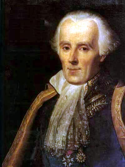
Principle of Insufficient Reason
- How to assign probability?
- \(n\) mutually exclusive, exhaustive outcomes
- Nothing distinguishes one from another
- Assign equal probability: \(p_i = 1/n\)
Example: Will the sun rise tomorrow?

- Unknown daily rate \(\theta\in[0,1]\); insufficient reason \(\Rightarrow\) uniform prior on \(\theta\)
- Every day is a success: after \(n\) rises, belief \(\propto\theta^{n}\)
- Predictive: \(P(\text{rises tomorrow})=\dfrac{n+1}{n+2}\)
- Sunrise for \(n=1{,}826{,}213\) days: odds \(1{,}826{,}214\) to one
- Laplace’s caveat: astronomy makes the true odds incomparably greater
Entropy Day by Day
Track differential entropy of the belief \(p(\theta)\) as sunrises arrive.
- Prior: \(p(\theta)=1\) on \([0,1]\) \(\Rightarrow\) \(H_0=0\)
- After \(n\) rises: \(p(\theta)=(n+1)\theta^{n}\)
- \(H_n=\dfrac{n}{n+1}-\log(n+1)\) (nats)
- Day \(n\) information gain: \(I_n=H_{n-1}-H_n=\log\!\left(1+\dfrac{1}{n}\right)-\dfrac{1}{n(n+1)}\)
From Insufficient Reason to MaxEnt
- Insufficient reason: uniform when we know only the outcomes (or only \(\theta\in[0,1]\))
- Rule of succession: same idea, after observing counts
- Jaynes: maximise \(H(p)\) subject to whatever we do know
- No extra constraints \(\Rightarrow\) MaxEnt recovers \(p_i = 1/n\)
- Mean energy (or other moments) \(\Rightarrow\) exponential family
Jaynes and Maximum Entropy
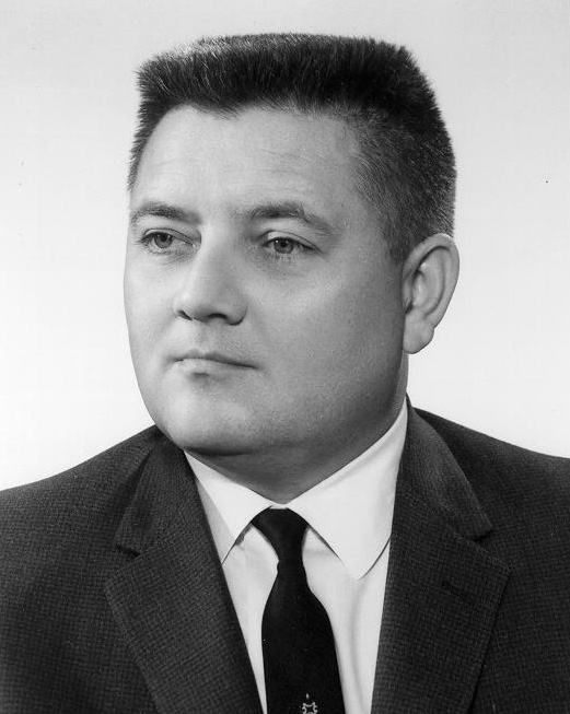
Maximum Entropy Motivation
- Jaynes (1957): Statistical mechanics as inference with incomplete information
- Maximum entropy principle: maximise uncertainty given constraints
- Avoids unwarranted assumptions beyond available data
Dice Example
- Dice example: Average result 4.5 instead of 3.5
- Constraints:
- \(\sum_{n=1}^6 P_n = 1\) (normalization)
- \(\sum_{n=1}^6 nP_n = 4.5\) (observed average)
Die Roll Simulation
Rolls: 0
Sample mean: —
H(p): —
Outcome weights (auto-normalised to probabilities)
Jaynes’ die (mean 4.5, not 3.5) is the running example. The same Lagrange move recovers physics and statistics.
- One constraint: mean energy \(\Rightarrow\) \(p_i \propto e^{-\beta E_i}\)
- Two constraints: mean and variance \(\Rightarrow\) Gaussian
- Lagrange multiplier on energy is coldness \(\beta\) from week 1
Derivation of the Boltzmann Distribution
For fixed mean energy \(U\), maximum entropy recovers Boltzmann weights. ::: incremental
- Constraints: \(\sum_i p_i = 1\) and \(\sum_i p_i E_i = U\)
- MaxEnt: \(p_i \propto e^{-\beta E_i}\) with coldness \(\beta = 1/k_B T\)
- Normalise: \(Z(\beta)=\sum_i e^{-\beta E_i}\), so \(p_i = e^{-\beta E_i}/Z\)
:::
MaxEnt Under Constraints: the Proof
This is the week’s main theorem: constrained MaxEnt \(\Rightarrow\) exponential family.
- Discrete \(x_i\); maximise \(H(p)=-\sum_i p_i\log p_i\)
- Constraints: \(\sum_i p_i=1\) and \(\sum_i p_i f_k(x_i)=\langle f_k\rangle\) for \(k=1,\ldots,m\)
- Lagrangian: \(\mathscr{L}=\sum_i p_i\log p_i + \lambda_0\bigl(\sum_i p_i-1\bigr)+\sum_k \lambda_k\bigl(\sum_i p_i f_k(x_i)-\langle f_k\rangle\bigr)\)
- Stationarity: \(\partial\mathscr{L}/\partial p_i=0\) \(\Rightarrow\) \(p_i\propto e^{-\sum_k \lambda_k f_k(x_i)}\)
- Write \(T_k(x_i)=f_k(x_i)\): sufficient statistics fixed by the constraints
- MaxEnt solution: \(p_i=\dfrac{e^{-\sum_k \lambda_k T_k(x_i)}}{Z}\) on the discrete support
- Exponential family: \(p(x\mid\boldsymbol{\theta})\propto \exp\bigl(\boldsymbol{\theta}\!\cdot\! T(x)-A(\boldsymbol{\theta})\bigr)\)
- Identification: \(\boldsymbol{\theta} = -\boldsymbol{\lambda}\) (natural parameters \(=\) minus Lagrange multipliers)
- \(A(\boldsymbol{\theta})=\log Z(-\boldsymbol{\theta})\); \(\langle T_k\rangle = \partial A/\partial\theta_k\)
The General Maximum-Entropy Formalism
\[ p_i = \frac{\exp(-\lambda_1 f_1(x_i) - \ldots - \lambda_m f_m(x_i))}{Z(\lambda_1,\ldots,\lambda_m)} \] \[ Z(\ldots) = \sum_{i=1}^n \exp(-\lambda_1 f_1(x_i) - \ldots - \lambda_m f_m(x_i)) \] \[ \langle f_k \rangle = -\frac{\partial}{\partial \lambda_k}\log Z(\lambda_1,\ldots,\lambda_m) \quad k=1,2,\ldots,m. \]
The Exponential Family
Exponential Families
- Exponential families: cornerstone of information theory
- Natural parameters give us clean geometry
- Connects probability, entropy, and Fisher information
Definition
\[ p(\mathbf{x} | \boldsymbol{\theta}) = \exp\left(\boldsymbol{\theta}^\top T(\mathbf{x}) - \mathcal{A}(\boldsymbol{\theta})\right) h(\mathbf{x}) \] * \(\boldsymbol{\theta}\): natural parameters * \(T(\mathbf{x})\): sufficient statistics * \(\mathcal{A}(\boldsymbol{\theta})\): log partition function * \(h(\mathbf{x})\): base measure
Why “Natural” Parameters?
- Natural parameters appear linearly in exponent
- Special geometric properties
- Clean connection to Fisher information
- Simplifies entropy calculations
The Log Partition Function as Cumulant Generator
\[ \mathcal{A}(\boldsymbol{\theta}) = \log \int \exp\left(\boldsymbol{\theta}^\top T(\mathbf{x})\right) h(\mathbf{x}) \, d\mathbf{x} \]}
Cumulants from Derivatives
- \(\nabla \mathcal{A}(\boldsymbol{\theta}) = \mathbb{E}[T(\mathbf{x})]\) (mean)
- \(\nabla^2 \mathcal{A}(\boldsymbol{\theta}) = \mathrm{Cov}[T(\mathbf{x})]\) (covariance)
- Higher derivatives give higher cumulants
Connection to Fisher Information
\[ G(\boldsymbol{\theta}) = \nabla^2 \mathcal{A}(\boldsymbol{\theta}) = \mathrm{Cov}_{\boldsymbol{\theta}}[T(\mathbf{x})] \] * R.A. Fisher: bounds estimation accuracy (Cramér-Rao) * Fisher information = Hessian of \(\mathcal{A}\) * Fisher information = Covariance of sufficient statistics * Defines geometry of information space * More details in next section
Entropy in Natural Coordinates
\[ H(\boldsymbol{\theta}) = \mathcal{A}(\boldsymbol{\theta}) - \boldsymbol{\theta}^\top \boldsymbol{\mu} \] where \(\boldsymbol{\mu} = \nabla \mathcal{A}(\boldsymbol{\theta})\)
Why Natural Parameters?
\[ \nabla_{\boldsymbol{\theta}} H = -G(\boldsymbol{\theta})\boldsymbol{\theta} \] * Key result for information dynamics * Terms involving \(\nabla \mathcal{A}\) cancel * Fisher information connects geometry to dynamics
Example: Multivariate Gaussian
Gaussian in Exponential Family Form
Gaussian as exponential family: * \(\boldsymbol{\theta} = \Sigma^{-1}\boldsymbol{\mu}\) (natural parameters) * \(T(\mathbf{x}) = \mathbf{x}\) (sufficient statistics) * \(\mathcal{A}(\boldsymbol{\theta}) = \frac{1}{2}\boldsymbol{\theta}^\top\Sigma\boldsymbol{\theta} + \frac{1}{2}\log|\Sigma|\)
Fisher Information for Gaussian
\[ G(\boldsymbol{\theta}) = \Sigma \] * Fisher information = covariance * \(G^{-1} = \Sigma^{-1}\) = precision * High variance → low Fisher info → harder estimation (looser Cramér-Rao) * Low variance → high Fisher info → easier estimation (tighter Cramér-Rao)
Example: Categorical Distribution
Categorical in Exponential Family Form
Categorical distribution: * \(\boldsymbol{\theta} = (\log \pi_1, \ldots, \log \pi_{K-1})\) * \(T(\mathbf{x}) = (x_1, \ldots, x_{K-1})\) (one-hot) * \(\mathcal{A}(\boldsymbol{\theta}) = \log\left(\sum_{k=1}^{K-1} e^{\theta_k} + 1\right)\)
Fisher Information for Categorical
\[ G_{ij} = \begin{cases} \pi_i(1-\pi_i) & i=j \\ -\pi_i\pi_j & i \neq j \end{cases} \] * Rare categories → low Fisher info * Uniform distribution → balanced information
Why Exponential Families Matter
Why exponential families matter: * Emerge from maximum entropy principles * Define information geometry * Sufficient statistics capture all information * Computationally tractable * Clean form for information dynamics
Looking Ahead
Next steps: * Natural parameters → coordinate system * Fisher information → information topography
* Entropy gradients → drive dynamics * \(\nabla H = -G(\boldsymbol{\theta})\boldsymbol{\theta}\) → key to everything
Softmax is MaxEnt with Features
- Two-level \(\Leftrightarrow\) Bernoulli
- \(\theta = -\beta\varepsilon\) or \(\mathrm{logit}(\pi)\)
- Same \(A(\theta)=\log(1+e^{\theta})\)
Features, Not Just the Outcome
\[ p(y\mid x)=\frac{\exp(\theta\cdot f(x,y))}{\sum_{y'}\exp(\theta\cdot f(x,y'))} \] * Constraint: expected features match the data * Same multipliers as the die
Maximum Likelihood is the Same Fit
- MaxEnt with features \(=\) softmax
- Softmax MLE \(=\) moment matching
- The die was \(f(x)=x\)
Two Spins, One Coupling
\[ p(s)\propto\exp(h_1 s_1+h_2 s_2+J s_1 s_2) \] * Constraints: \(\langle s_1\rangle\), \(\langle s_2\rangle\), \(\langle s_1 s_2\rangle\) * \(J\) is the multiplier on a correlation
The Same Hamiltonian, Two Readings
- Physics: two interacting moments
- ML: a two-unit Boltzmann machine
- Inverse Ising \(=\) match the moments
The Legendre Transform
- Week 2: \(F = U - TS\)
- Same subtraction, new name
- Why the exponential family has two charts
Swap the Independent Variable
\[ y = \phi'(x),\qquad \phi^*(y) = xy - \phi(x) \] * Convex \(\phi\): the slope is a coordinate * \(\phi^*\) is the same information, different argument * The pair inverts: \(x = (\phi^*)'(y)\)
Helmholtz Was the First Example
- \(U(S,V,N)\): energy as a function of entropy
- \(T = \partial U/\partial S\): the slope
- \(F(T,V,N) = U - TS\): same physics, bath coordinates
Helmholtz Versus Gibbs
- Potential \(\leftrightarrow\) which variables the bath fixes
- \(F(T,V,N)=U-TS\): fixed \(T\), fixed volume (our setting; \(Z\))
- \(G(T,P,N)=F+PV=H-TS\): fixed \(T\), fixed pressure (chemistry; \(\mu\))
Entropy as Conjugate of the Log-Partition
\[ \boldsymbol{\eta} = \nabla A(\boldsymbol{\theta}),\qquad H = A(\boldsymbol{\theta}) - \boldsymbol{\theta}\cdot\boldsymbol{\eta} \] * \(A\) is convex: Hessian \(=\) Fisher \(=\) covariance * \(A^*(\boldsymbol{\eta}) = \boldsymbol{\theta}\cdot\boldsymbol{\eta} - A = -H\) * Same move as \(F = U - TS\)
Bernoulli: Check the Arithmetic
Bernoulli: \(\theta = \mathrm{logit}(p)\), \(A = \log(1+e^{\theta})\), \(\eta = p\) \[ H = A - \theta p = -p\log p -(1-p)\log(1-p) \] * If the subtraction misses \(H\), the signs are wrong
Two Charts, Named for Later
- \(\boldsymbol{\theta}\): \(e\)-coordinates (natural parameters)
- \(\boldsymbol{\eta}\): \(m\)-coordinates (moments)
- Dual flatness: week 6
- \(m\)-projection: week 7
Three Perspectives
Same \(H\); three operational assumptions about what probability is over.
- Carnot/Clausius: a heat engine — efficiency and the second law
- Shannon: a code — capacity and compression
- Szilard/Landauer: a bit in memory — \(k_B T \ln 2\) work and erasure
- Boltzmann/Gibbs: a macrostate at equilibrium
- Jaynes/Bayes: a state of knowledge under constraint
- All four layers: \(H\) forbids, \(p\) prescribes
- Carnot/Clausius: engines and the second law
- Shannon: a code
- Szilard/Landauer: a bit in memory
- Boltzmann: a macrostate
- Jaynes: a state of knowledge
- All layers: \(H\) forbids, \(p\) prescribes
Define This Week
- What is the maximum entropy principle?
- What is the exponential family?
- What is the Legendre transform?
- How is entropy understood today?
Named, Not Yet Answered
- MaxEnt over a coupling, not a list of moments? (week 8)
After This Lecture
- Quiz 2: 10 November, first ten minutes
Further Reading
the whole paper of Jaynes (1957)
Chapter 22 of MacKay (2003)
Chapter 12 of Cover and Thomas (1991)
Chapters 11–12 of Jaynes (2003)
Exercises 22.12–22.13 of MacKay (2003)
the whole paper of Berger et al. (1996)
the original one-dimensional model of Ising (1925)
Boltzmann machines of Ackley et al. (1985)
pairwise MaxEnt on a retina of Schneidman et al. (2006)
Section 1.5.5 and Chapter 5 of Welling et al. (2026)
Thanks!
- company: Trent AI
- book: The Atomic Human
- twitter: @lawrennd
- The Atomic Human
- newspaper: Guardian Profile Page
- blog: http://inverseprobability.com