

Week 3: Shannon Entropy and the Partition Function
[jupyter][google colab][reveal][edit]
Abstract:
In this lecture we cover Shannon entropy as a measure of uncertainty, and its mathematical relationship to thermodynamic entropy. We show that the partition function as a generating function. We introduce mutual information, \(I\), channel capacity, and the data-processing inequality (DPI) are introduced as results. \(I\) and DPI are proved in week 8.
No class test today. Boltzmann and free energy were last week. Today: Shannon \(H\) and the partition function as a generating function.
This Session
Time plan (120 minutes)
| Minutes | Block |
|---|---|
| 0–10 | Recap Boltzmann / free energy; preview Maxwell (next week) |
| 10–40 | Shannon axioms; Wiener from Gibbs; equivalence to Boltzmann |
| 40–55 | Arithmetic coding (MacKay Ch.~6) then Dasher |
| 55–65 | Break |
| 65–100 | Canonical ensemble; \(Z\) as generating function; bath revisited |
| 100–120 | KL-divergence; Chain rule; define \(I(X;Y)\); capacity (statement); DPI (statement) |
Week 1 introduced Shannon’s portrait and embodiment factors in bits per second. This lecture derives \(H=-\sum_i p_i\log p_i\) and shows that Boltzmann entropy uses the same functional form. The human–machine bandwidth gap is a communication bottleneck; channel capacity is the analogous no-go on codes, not on embodiment.
Information, energy and intelligence course notebook setup
We install some bespoke code for creating and saving plots as well as loading data sets.
import importlib.utilcmd = install_command('pods')%system {cmd}cmd = install_command('notutils')%system {cmd}cmd = install_command('mlai')%system {cmd}Shannon Entropy
Information Theory and AI
The idea behind this course is to proper understand the relationship between human and machine intelligence (and perhaps also the natural intelligences around us) we should step back from notions of rankable intelligence (which have their origins in eugenics) and towards more fundamental ideas which we can measure and rank, in particular information theory.
Claude Shannon was an American mathematician. He developed his notion of information thoery when he was working at Bell Labs (Shannon, 1948a). His objective was to understand how to make the most efficient use of resources when building out the telephone network. His idea was to model the telephone exchange as a digital system. Shannon is known to have spent considerable time talking to Norbert Wiener (Conway and Siegelman, 2005) whose own ideas about information came from his notion of what he called a theory of ignorance (Wiener, 1953). Wiener’s notions were inspired by Willard Gibbs’ work on entropy. Shannon built on Wiener’s ideas in two important ways. Firstly he considered discrete distributions (Gibbs entropies are tyipcally continuous entropies) and secondly he removed the context from the mathematics.
This removal of context is particularly important philosophically, to my mind perhaps the most important conceptual contribution from Shannon. It’s important because it makes information fungible. That allows us to compare information transfer rates across different types of processing entities.
See Lawrence (2024) p. . See Lawrence (2024) p. .
A typical human, when speaking, shares information at around 2,000 bits per minute. Two machines will share information at 600 billion bits per minute. In other words, machines can share information 300 million times faster than us. This is equivalent to us traveling at walking pace, and the machine traveling at the speed of light.
From this perspective, machine decision-making belongs to an utterly different realm to that of humans. Consideration of the relative merits of the two needs to take these differences into account. This difference between human and machine underpins the revolution in algorithmic decision-making that has already begun reshaping our society Lawrence (2024).
Brownian Motion and Wiener
Robert Brown was a botanist who was studying plant pollen in 1827 when he noticed a trembling motion of very small particles contained within cavities within the pollen. He worked hard to eliminate the potential source of the movement by exploring other materials where he found it to be continuously present. Thus, the movement was not associated, as he originally thought, with life.
In 1905 Albert Einstein produced the first mathematical explanation of the phenomenon. This can be seen as our first model of a ‘curve of a simple molecule of air.’ To model the phenomenon Einstein introduced stochasticity to a differential equation. The particles were being peppered with high-speed water molecules, that was triggering the motion. Einstein modelled this as a stochastic process.
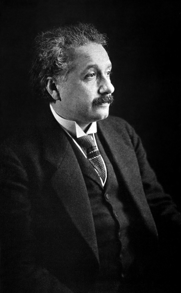
Figure: Albert Einstein’s 1905 paper on Brownian motion introduced stochastic differential equations which can be used to model the ‘curve of a simple molecule of air.’
Norbert Wiener was a child prodigy, whose father had schooled him in philosophy. He was keen to have his son work with the leading philosophers of the age, so at the age of 18 Wiener arrived in Cambridge (already with a PhD). He was despatched to study with Bertrand Russell but Wiener and Russell didn’t get along. Wiener wasn’t persuaded by Russell’s ideas for theories of knowledge through logic. He was more aligned with Laplace and his desire for a theory of ignorance. In is autobiography he relates it as the first thing he could see his father was proud of (at around the age of 10 or 11) (Wiener, 1953).
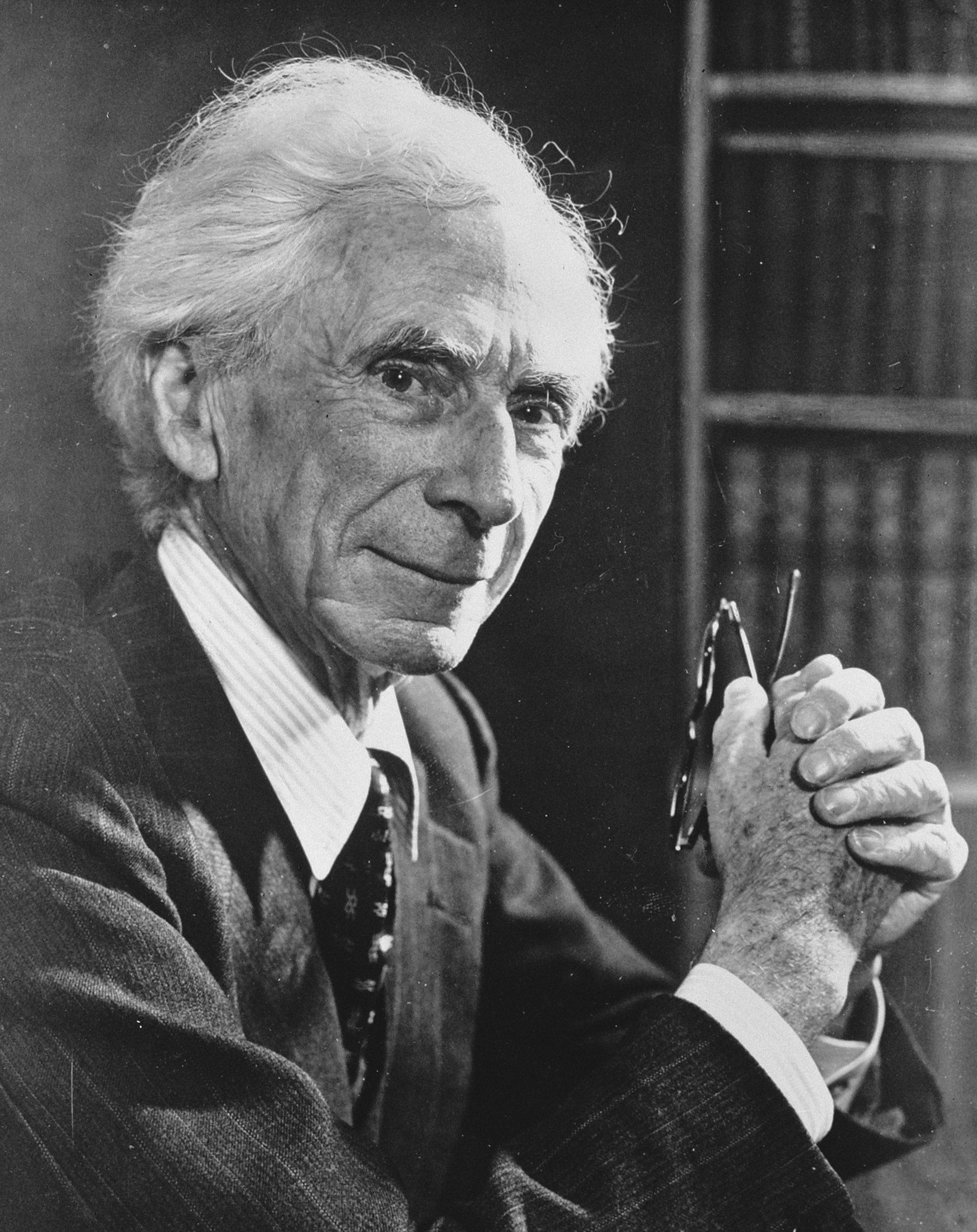
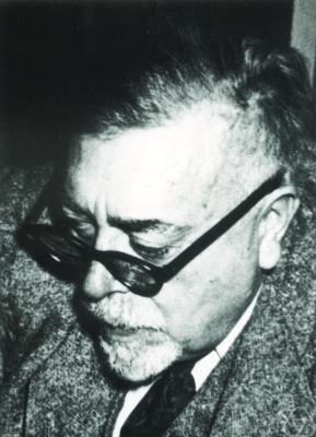
Figure: Bertrand Russell (1872-1970), Albert Einstein (1879-1955), Norbert Wiener, (1894-1964)
But Russell (despite also not getting along well with Wiener) introduced Wiener to Einstein’s works, and Wiener also met G. H. Hardy. He left Cambridge for Göttingen where he studied with Hilbert. He developed the underlying mathematics for proving the existence of the solutions to Einstein’s equation, which are now known as Wiener processes.
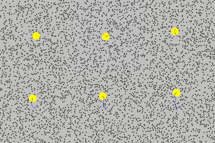
Figure: Brownian motion of a large particle in a group of smaller particles. The movement is known as a Wiener process after Norbert Wiener.
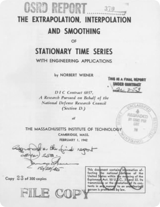
Figure: Norbert Wiener (1894 - 1964). Founder of cybernetics and the information era. He used Gibbs’s ideas to develop a “theory of ignorance” that he deployed in early communication. On the right is Wiener’s wartime report that used stochastic processes in forecasting with applications in radar control (image from Coales and Kane (2014)).
Wiener himself used the processes in his work. He was focused on mathematical theories of communication. Between the world wars he was based at Massachusetts Institute of Technology where the burgeoning theory of electrical engineering was emerging, with a particular focus on communication lines. Winer developed theories of communication that used Gibbs’s entropy to encode information. He also used the ideas behind the Wiener process for developing tracking methods for radar systems in the second world war. These processes are what we know of now as Gaussian processes (Wiener (1949)).
Shannon Entropy from Axioms
Shannon entropy \(H=-\sum_i p_i\log p_i\) measures uncertainty. Thermodynamic entropy \(S=kH\) uses the same functional form with a different operational reading: \(H\) bounds what a code cannot do; the distribution \(p\) is the prescription — the code or the belief.
Figure: Binary entropy is maximal at \(p=\frac12\) and falls as the source becomes predictable.
import numpy as npdef shannon_entropy(probs, base=2):
p = np.asarray(probs, dtype=float)
p = p[p > 0]
H = -np.sum(p * np.log(p))
return H / np.log(base) if base == 2 else H
# Worksheet 1 tabulates fair coin, p=0.9, uniform-8, Boltzmann at beta=1Arithmetic Coding and Dasher
Arithmetic Coding
In Chapter 6 of Information Theory, Inference, and Learning Algorithms (MacKay, 2003), MacKay introduces arithmetic coding with a clear philosophy: compression of data from a source entails probabilistic modelling of that source. The encoding operation is then almost an afterthought — once you can predict, you can code.
The guessing game
Section 6.1 motivates the idea with a guessing game. An English speaker tries to predict the next character of a text; after each correct guess we record how many attempts it took. The sequence of guess-counts is highly skewed toward 1 and 2, so it compresses easily. Decoding needs an identical twin who makes the same sequence of guesses: stop them after the recorded number of attempts and they land on the right letter.
The game demonstrates two design principles we will keep: (i) a time-varying predictive mapping is allowed — the predictor may use as much context as it likes; (ii) encoder and decoder must share an identical model.
From guesses to intervals
Section 6.2 replaces the human by a program that, given the string so far, returns a predictive distribution \(\{p_i\}\) over the next symbol. Arithmetic coding turns that distribution into nested intervals on \([0,1)\) (Figures 6.1–6.2). A binary transmission itself defines an interval — the string 01 is the dyadic interval \([0.25, 0.50)\) — so encoding means: find a bit-string whose interval sits inside the interval that the model assigned to the message.
MacKay’s Algorithm 6.3 is the iterative form. Write \(Q_n\) and \(R_n\) for the lower and upper cumulative predictive probabilities. Starting from \(u=0\), \(v=1\), \(p=v-u\), each symbol updates \[ v \leftarrow u + p\,R_n(x_n\mid x_{<n}),\qquad u \leftarrow u + p\,Q_n(x_n\mid x_{<n}),\qquad p \leftarrow v-u. \] The Shannon information content of the string is \(h(x\mid H)=\log[1/P(x\mid H)]\); Exercise 6.1 shows the coded length stays within two bits of that ideal.
import json
import math
from collections import defaultdict
First the predictive model. Arithmetic coding does not prescribe how predictions are made — only that encoder and decoder agree. For Dasher we use a unigram–bigram blend \(P(c \mid c') \propto w\,P_{\mathrm{bi}}(c \mid c') + (1-w)\,P_{\mathrm{uni}}(c)\).
corpus = """
Alice was beginning to get very tired of sitting by her sister on the bank,
and of having nothing to do: once or twice she had peeped into the book her
sister was reading, but it had no pictures or conversations in it.
"""
model = train_from_text(corpus, bigram_weight=0.82)
print(f"H(next | ∅)    = {model.entropy_rate(''):.3f} bits/char")
print(f"H(next | 't')  = {model.entropy_rate('t'):.3f} bits/char")
print(f"H(next | 'th') = {model.entropy_rate('th'):.3f} bits/char")
After th the predictive mass concentrates on e, so the conditional entropy drops. That drop is the tall e box in Dasher.
The helpers below follow MacKay’s Algorithm 6.3 and Figure 6.1: narrow \([u,v)\subseteq[0,1)\), then pick a dyadic bit-string inside it. The decoder is the identical twin — same predictions, ask which symbol interval contains the number defined by the bits.
message = normalise_text("the rabbit")
u, v, ideal_bits = encode_interval(message, model)
bitstring, _ = encode(message, model)
recovered = decode(bitstring, len(message), model)
print(f"message:   {message!r}")
print(f"[u, v)  = [{u:.6f}, {v:.6f})  width={v-u:.3e}")
print(f"ideal:     {ideal_bits:.3f} bits  "
      f"({ideal_bits / len(message):.3f} bits/char)")
print(f"bitstring: {bitstring}  ({len(bitstring)} bits)")
print(f"decoded:   {recovered!r}  ok={recovered == message}")
for step in interval_trace(message, model)[:4]:
    print(f"  '{step['char']}': p={step['p']:.3f}  "
          f"bits={step['bits']:.2f}  "
          f"[u,v)=[{step['u']:.4f},{step['v']:.4f})")
uniform = len(message) * math.log2(len(model.chars))
print(f"uniform: {uniform:.3f} bits "
f"({uniform / len(message):.3f} bits/char)")
print(f"saving: {uniform - ideal_bits:.3f} bits vs uniform")Compare with a uniform code over the same alphabet. A model that knows English beats uniform — and the gap is exactly what good prediction buys you.
Dasher (Ward et al., 2000; MacKay-dasher98?) draws Algorithm 6.3: each letter is a vertical interval whose height is its predictive probability, and zooming into a letter is the update \((u,v)\leftarrow(u+pQ,\,u+pR)\). Write the trained tables to JSON; point the canvas at your file (or replace the default dasher-lm.json) and the box sizes become your \(P(c\mid\mathrm{context})\).
write_dasher_lm(model, "dasher-lm.json")
print(sorted(model.to_dasher_dict().keys()))
For a one-shot shell export from the talks tree (same logic as the helpers above):
python arithmetic_coding.py path/to/corpus.txt \
    -o scripts/dasher/dasher-lm.json --demo
Dasher: Arithmetic Coding as Interface
Dasher is a writing interface invented by David MacKay (MacKay-dasher98?) that visualises the connection between arithmetic coding and character prediction. Having seen MacKay’s Algorithm 6.3 — nested intervals on \([0,1)\) whose lengths are predictive probabilities (MacKay, 2003, p. Ch.~6). If we arrange a character set vertically with each character occupying space proportional to its probability, then selecting a character is equivalent to zooming into its interval in the arithmetic code.
Moving the mouse to the right zooms toward whichever letter the cursor is pointing at. Because common letters (e, t, a, space) have large probability, they occupy large screen area — they are easy to aim at. Rare letters (q, z, x) have tiny probability, occupy smaller screen area, and are correspondingly hard to hit. Ease of selection equals low information content, which equals efficiency.
If you select “th,” notice how ‘e’ grows to dominate the display. It’s hard to select ‘q,’ a rarer letter, but if you do ‘u’ dominates the next box. The visualisation makes the language model’s predictions tangible.
DASHER
bits: 0.0 avg: — b/ch H(next): —
Click or Space to Go/Pause · Copy extracts text · pointer right zooms · left zooms out · Backspace unwrites · Escape resets
Figure: Dasher: continuous-zoom arithmetic coding interface. Move the pointer right of centre — boxes enlarge and stream left across the crosshair. Character height is proportional to \(P(\texttt{char} | \texttt{context})\). Try “th”: after ‘t’ and ‘h,’ ‘e’ swells to dominate the display.
Dasher is the pair in one interface. Letter height is \(p(\text{char}\mid\text{context})\); the information cost of a hit is \(-\log p\). \(H(\text{next})\) is the no-go on the remaining rate. The language model is the prescription: this is the next letter you should make easy to hit. The bits-per-second counter is the same unit as lecture 1’s bandwidth bottleneck — here spent on a pointer, not on speech.
The Partition Function
The partition function \(Z(\beta)=\sum_i e^{-\beta E_i}\) is a generating function: \(U=-\partial_\beta\log Z\), \(F=-\beta^{-1}\log Z\), \(S=\beta(U-F)\). The canonical ensemble is an equilibrium construction; driving in finite time leaves that manifold.
Figure: Thermodynamic quantities from \(Z(\beta)\) for the two-state system used as a running example.
import numpy as np

def partition(energies, beta):
    return np.sum(np.exp(-beta * np.asarray(energies)))

def thermo_from_Z(beta, energies):
    e = np.asarray(energies, dtype=float)
    Z = partition(e, beta)
    p = np.exp(-beta * e) / Z
    U = np.sum(p * e)
    F = -np.log(Z) / beta
    S = beta * (U - F)
    return U, S, F
GAIST on Entropy and the Partition Function
Section 1.2.3 of (Welling et al., 2026) defines Shannon entropy as expected surprisal, \(\mathrm{S}[p] = -\int p\log p\), in nats. It computes the Gaussian entropy and shows that it depends only on \(\sigma\), not on \(\mu\). Section 1.2.4 introduces KL as relative entropy, the information lost when \(q\) stands in for \(p\), and records the chain-rule decomposition of KL. That is useful scaffolding for week 6; it is not Shannon’s chain rule for \(H\).
Section 3.2.4 is the generating-function half of today’s lecture: from \(Z\) to mean energy, entropy, and free energy. Read those two sections. Do not look here for the Shannon axioms, for \(S = kH\), or for channel capacity. Those are MacKay and Shannon (1948). GAIST treats entropy as a property of a distribution, not as a no-go on a code.
GAIST §1.2.3 uses \(-\int p\log p\) for Gaussians — that is differential entropy. It can be negative and is not bounded like discrete Shannon \(H\in[0,\log n]\). Below we introduce KL divergence, which is always \(\ge 0\) discrete and continuous. That is why MaxEnt projections minimise \(\text{KL}(\cdot\|r)\), not raw \(H\).
Discrete Shannon Entropy Is Bounded
KL divergence measures information lost when \(q\) is used instead of \(p\). It is non-negative in both discrete and continuous settings (with common support). Unlike Shannon entropy, it is defined relative to a reference. MaxEnt and \(m\)-projections minimise \(\text{KL}(\cdot\|r)\); that is why week 4’s die optimisation used \(\sum_i p_i\log(p_i/r_i)\).
For \(\mathcal{N}(0,\sigma^2)\), differential entropy is \(\frac{1}{2}\log(2\pi e\sigma^2)\) in nats. As \(\sigma\to 0\) it diverges negatively. Discrete Shannon entropy stays in \([0,\log n]\). Thermodynamic \(S=kH\) in week 1 used the discrete sum form on Boltzmann probabilities. Continuous MaxEnt still works because constraints fix scale; comparing to a reference uses KL, which remains non-negative.
Figure: Left: binary Shannon entropy is bounded. Right: Gaussian differential entropy can be negative.
Scaffolding, Not Outcomes
The chain rule \(H(X,Y)=H(X)+H(Y|X)\) is the algebraic source of multi-information. Mutual information \(I(X;Y)=H(X)-H(X|Y)\) is the pairwise case; we do not yet treat \(n>2\). Channel capacity \(C\) is a no-go on rate; the capacity-achieving input distribution is the prescription. The data-processing inequality is the no-go on \(I\): processing cannot create information. Cover and Thomas Theorem 2.8.1 is the reading; the proof waits for week 8, when \(I\) is first-class.
Figure: Mutual information for a binary symmetric channel; capacity is achieved at uniform input.
Three Framings, First Pass
Information, thermodynamic, and Bayesian readings of the same \(H\) differ in what the probability is over and who is inferring. The intended comparison is LO7 in week 4.
Define This Week
Interpret later: how entropy is understood today (week 5, then week 8); chain rule as the source of multi-information (week 8). DPI is named today; define-stage proof is week 8.
After This Lecture
Next week: Maxwell’s demon and Landauer. LLM exercise: ask whether Shannon entropy is a bound or a recipe.
Further Reading
Sections 1–6 of Shannon (1948b)
Chapters 1–4; Chapter 6 of MacKay (2003)
Chapter 2 of Cover and Thomas (1991)
Sections 1.2.3–1.2.4 and 3.2.4 of Welling et al. (2026)
Chapter 16 of Callen (1985)
Chapter 7 of Cover and Thomas (1991)
Chapters 8–10 of MacKay (2003)
Thanks!
For more information on these subjects and more you might want to check the following resources.
- company: Trent AI
- book: The Atomic Human
- twitter: @lawrennd
- podcast: The Talking Machines
- newspaper: Guardian Profile Page
- blog: http://inverseprobability.com