

Week 1: Introduction, Probability Review, and Motivation
[jupyter][google colab][reveal][edit]
Abstract:
In this lecture we motivate the course and describe the mechanics of delivery. That will involve a review of Laplace’s demon and Laplace’s gremlin. The aim is to centre the notion of uncertainty in the material. We’ll also how we would like to see you deploy that in your course worksheets, where marks will be given for answers that demonstrate the type of skepticism we see in the Socratic method. We will give a brief review of probability and then introduce entropy. We will relate energy to probability through the way the term energy is used in machine learning, which is typically in the form of a “thermodynamic” or “Gibbs” energy rather than a mechanical Hamiltonian. The difference between these will also be explained. We will release Worksheet 1 that will need to be submitted before lecture starts in Week 2.
First meeting. FW26. Two hours from 10:00; no class test. Worksheet 1 (Socratic dialogue) is released and due by 10:00 at the start of lecture 2 (20 October). Quiz 1 is also at the start of lecture 2: probability, elementary entropy, and the Week 1 seeds.
This Session
Time plan (120 minutes)
| Minutes | Block |
|---|---|
| 0–15 | Course mechanics; questions list; the motivation and theme |
| 15–35 | ‘Socratic’ approach: curiosity, skepticism, submission rules |
| 35–65 | Probability review: product/sum/Bayes; basic distributions |
| 65–75 | Break |
| 75–95 | Entropy review (elementary \(H\)); bits and nats |
| 95–110 | Energy in ML; motivation and bandwidth; Boltzmann seed |
| 110–118 | Culmination: potential → stochastic → kinetic? → Hamiltonian / HMC |
| 118–120 | Worksheet 1 brief; Quiz 1 preview |
Course Mechanics
Eight lectures, Tuesdays, this room. Four in-class Moodle quizzes, ten minutes, at the start of lectures 2, 5, 7 and 8. Students need a device. No notes, no network, no LLMs during the quiz. Four take-home worksheets. Worksheet 1 is a Socratic LLM dialogue plus reflection; later worksheets mix code and shorter LLM probes using the same curiosity–skepticism habit. Worksheets are released in lectures 1, 4, 6 and 7 and due at the start of lectures 2, 5, 7 and 8 respectively.
Questions We Will Return To
The questions page is published today. Students should meet the whole list. They should not expect to answer most of it. Two stages: define (textbook answer, usually this week or the week the object is introduced) and interpret (the course’s own reading, often week 5 or week 8).
Information, energy and intelligence course notebook setup
We install some bespoke code for creating and saving plots as well as loading data sets.
import importlib.utilcmd = install_command('pods')%system {cmd}cmd = install_command('notutils')%system {cmd}cmd = install_command('mlai')%system {cmd}Motivation
Perpetual Motion and Superintelligence
Imagine in 1925 a world where the automobile is already transforming society, but big promises are being made for things to come. The stock market is soaring, the 1918 pandemic is forgotten. And every major automobile manufacturer is investing heavily on the promise they will each be the first to produce a car that needs no fuel. A perpetual motion machine.
Well, of course that didn’t happen. But I sometimes wonder if what we’re seeing today 100 years later is the modern equivalent of that. In 2026 billions are being invested in promises of superintelligence and artificial general intelligence that will transform everything.
We know why perpetual motion is impossible: the second law of thermodynamics tells us that entropy always increases. So we can’t have motion without entropy production. No matter how clever the design, you cannot extract energy from nothing, and you cannot create a closed system that does useful work indefinitely without an external energy source.
How might we make an equivalent statement for the bizarre claims around superintelligence? Some inspiration comes from Maxwell’s demon, an “intelligent” entity which operates against the laws of thermodynamics. The inspiration comes because the demon suggests that for the second law to hold there must be a relationship between the demon’s decisions and thermodynamic entropy.
One of the resolutions comes from Landauer’s principle, the notion that erasure of information requires heat dissipation. This suggests there are fundamental information-theoretic constraints on intelligent systems, just as there are thermodynamic constraints on engines.
I’ve no doubt that AI technologies will transform our world just as much as the automobile has. But I also have no doubt that the promise of unconstrained superintelligence is just as silly as the promise of perpetual motion.
Pierre-Simon Laplace
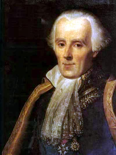
Figure: Pierre-Simon Laplace 1749-1827.
Laplace’s Determism
Figure: Laplace’s determinism book reference.
Famously, Laplace considered the idea of a deterministic Universe, one in which the model is known, or as the below translation refers to it, “an intelligence which could comprehend all the forces by which nature is animated.” He speculates on an “intelligence” that can submit this vast data to analysis and propsoses that such an entity would be able to predict the future.
Given for one instant an intelligence which could comprehend all the forces by which nature is animated and the respective situation of the beings who compose it—an intelligence sufficiently vast to submit these data to analysis—it would embrace in the same formulate the movements of the greatest bodies of the universe and those of the lightest atom; for it, nothing would be uncertain and the future, as the past, would be present in its eyes.
This notion is known as Laplace’s demon or Laplace’s superman.
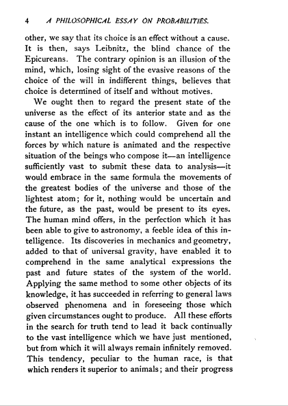
Figure: Laplace’s determinsim in English translation.
Laplace’s Gremlin
Unfortunately, most analyses of his ideas stop at that point, whereas his real point is that such a notion is unreachable. Not so much superman as strawman. Just three pages later in the “Philosophical Essay on Probabilities” (Laplace, 1814), Laplace goes on to observe:
The curve described by a simple molecule of air or vapor is regulated in a manner just as certain as the planetary orbits; the only difference between them is that which comes from our ignorance.
Probability is relative, in part to this ignorance, in part to our knowledge.
Figure: Laplace’s gremlin in the original French.
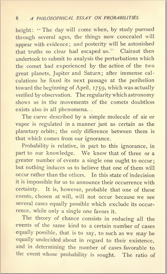
Figure: To Laplace, determinism is a strawman. Ignorance of mechanism and data leads to uncertainty which should be dealt with through probability.
In other words, we can never make use of the idealistic deterministic Universe due to our ignorance about the world, Laplace’s suggestion, and focus in this essay is that we turn to probability to deal with this uncertainty. This is also our inspiration for using probability in machine learning. This is the true message of Laplace’s essay, not determinism, but the gremlin of uncertainty that emerges from our ignorance.
The “forces by which nature is animated” is our model, the “situation of beings that compose it” is our data and the “intelligence sufficiently vast enough to submit these data to analysis” is our compute. The fly in the ointment is our ignorance about these aspects. And probability is the tool we use to incorporate this ignorance leading to uncertainty or doubt in our predictions.
Laplace’s Gremlin
The curve described by a simple molecule of air or vapor is regulated in a manner just as certain as the planetary orbits; the only difference between them is that which comes from our ignorance. Probability is relative, in part to this ignorance, in part to our knowledge. We know that of three or greater number of events a single one ought to occur; but nothing induces us to believe that one of them will occur rather than the others. In this state of indecision it is impossible for us to announce their occurrence with certainty. It is, however, probable that one of these events, chosen at will, will not occur because we see several cases equally possible which exclude its occurrence, while only a single one favors it.
— Pierre-Simon Laplace (Laplace, 1814), pg 5
The representation of ignorance through probability is the true message of Laplace, I refer to this message as “Laplace’s gremlin,” because it is the gremlin of uncertainty that interferes with the demon of determinism to mean that our predictions are not deterministic.
Our separation of the uncertainty into the data, the model and the computation give us three domains in which our doubts can creep into our ability to predict. Over the last three lectures we’ve introduced some of the basic tools we can use to unpick this uncertainty. You’ve been introduced to, (or have yow reviewed) Bayes’ rule. The rule, which is a simple consequence of the product rule of probability, is the foundation of how we update our beliefs in the presence of new information.
The real point of Laplace’s essay was that we don’t have access to all the data, we don’t have access to a complete physical understanding, and as the example of the Game of Life shows, even if we did have access to both (as we do for “Conway’s universe”) we still don’t have access to all the compute that we need to make deterministic predictions. There is uncertainty in the system which means we can’t make precise predictions.
Gremlins are imaginary creatures used as an explanation of failure in aircraft, causing crashes. In that sense the Gremlin represents the uncertainty that a pilot felt about what might go wrong in a plane which might be “theoretically sound” but in practice is poorly maintained or exposed to conditions that take it beyond its design criteria. Laplace’s gremlin is all the things that your model, data and ability to compute don’t account for bringing about failures in your ability to predict. Laplace’s gremlin is the uncertainty in the system.

Figure: Gremlins are seen as the cause of a number of challenges in this World War II poster.
Probability Review
Notation: we often write \(P(x,y)\) for \(P(X=x,Y=y)\). Unlike a generic bivariate function, \(P(x,y)=P(y,x)\).
The product rule relates joint and conditional. The sum rule recovers a marginal by summing out the variable you do not care about. Continuous analogues replace sums by integrals.
Bayes is not a third axiom; it is the product rule rearranged. The barrels example below is a small discrete inversion of the conditioning.
Work the numbers on the board if time allows. The same pattern applies to coins, medical tests, or any two-hypothesis discrete update.
Quiz 1 will ask a small discrete Bayes inversion (barrels, coins, two hypotheses) and recognition of the named distributions below.
Common Distributions
These are prerequisites restated, not new theory. Several of them reappear later as maximum-entropy distributions under moment constraints.
A fair coin is Bernoulli(\(1/2\)). A two-state thermal system with fixed energies is Bernoulli once occupation probabilities are written down.
Poisson Distribution
Figure: The Poisson distribution.
Differential entropy of a Gaussian grows with \(\sigma\) and can be negative. For a review, recognise the density and the two parameters.
The Gaussian Density
The Gaussian density is perhaps the most commonly used probability density. It is defined by a mean, \(\mu\), and a variance, \(\sigma^2\). The variance is taken to be the square of the standard deviation, \(\sigma\).
\[\begin{align} p(y| \mu, \sigma^2) & = \frac{1}{\sqrt{2\pi\sigma^2}}\exp\left(-\frac{(y- \mu)^2}{2\sigma^2}\right)\\& \buildrel\triangle\over = \mathscr{N}\left(y|\mu,\sigma^2\right) \end{align}\]
Figure: The Gaussian PDF with \({\mu}=1.7\) and variance \({\sigma}^2=0.0225\). Mean shown as red line. It could represent the heights of a population of students.
Doubt
What Laplace’s gremlin implies in practice is that we can never be certain about outcome, so doubt is an inevitable consequence of our lack of knowledge. It is what drives us to develop quantitative notions for uncertainty. We have already introduced probability, but the main focus of the course will be entropy. The concept that unifies information and entropy, and therefore we argue (perhaps) intelligence.
We will look to apply these ideas to how we approach our learning as well as what we learn. Bringing doubt into your own reasoning is a way in which you can develop your understanding. Learning to express that doubt through challenging a statement. The model we will use finds its origins in Socrates.
Worksheets and LLMs: Can you be Socrates?
The general approach we’d like to take to this course is that of a “community of inquiry” (see Chapter 4, Lipman (2012)). The unusual modern twist on this notion is that the LLMs themselves become part of that community.
Each of us will have different perspectives on what an LLM does and does not provide. You are welcome to bring those perspectives into your work. In particular, for each worksheet, you will be asked to reflect on the LLM responses and the process. Part of that reflection should be specific to the exercise and what you learnt about the subject. But I would like part of that reflection to be general about your understanding of the LLM and what it does and doesn’t provide. For worksheets 2, 3, and 4 a portion of that reflection will be on how you feel your understanding of LLMs as a tool of inquiry has evolved (if it evolved!).
The assessment model is based on is 1. a form of questioning enquiry generally called “the Socratic method” is an informative way of exploring a topic 2. an impression that the current generation of LL models is weak when asked to sustain Socratic dialogue. Answers tend to be expansive and when read carefully can lead to ‘diaclectic vertigo’ 3. The new idea we’re testing “Socratic method” can be deployed by reversing the role of Socrates and the student.
So in other words we are asking you to take on the role of Socrates in these conversations.
The general background is an idea that in order to develop your understanding of a subject through interaction with an LLM you need two components to your enquiry: curiousity and skepticism. The curiousity allows you to generate the prompt and the LLM to regurgitate some of its knowled (or perform searches that it summarises). But the skepticism engages with that summary through challenging the conclusions that the LLM has. In the Socratic elenchus that challenge is through pointing out a logical inconsistency that arises (Vlastos (1993)), perhaps through a side implication. For our purpose that challenge may not take exactly that form. But it should push back on the narrative the LLM provides. Generating such push back also requires you to engage with the material the LLM has provided.
For Socrates these are curated dialogues (written by Plato, e.g. Plato (1914)). So its normally the case that his challenges hit home. In your case, that won’t normally be the case. And we don’t expect you to curate your dialogue. What we’d like instead is a period of inquiry that is then summarised by a single dialogue that is played out with one LLM in a short session of 10 prompts and responses.
Classical Socratic practice (elenchus) tests consistency by questioning, not by lecturing. Contemporary seminar pedagogy keeps the same habit: the questioner holds the inquiry. Current LLMs default to exposition and agreement; they rarely sustain adversarial follow-ups without being steered. Assigning the student the Socrates role forces engagement with the subject matter rather than passive acceptance of a fluent summary.
Dialectical Vertigo
In the book, The Grasshopper (Suits, 1978), the eponymous protaganist, Grasshopper, asks his student, Skepticus, to take on this role.
What you are describing, Skepticus, is a chronic but minor ailment of philosophers. It is called dialectical vertigo, and its cure is the immediate application of straightforward argumentation.
The Grasshopper to Skepticus in The Grassohopper: Games, Life and Utopia (Suits, 1978 pg 37)
Worksheets are marked with 5 points for curiosity, 5 for skepticism, and 5 points for the reflection (15% of the module). You will be provided with a markdown template for your answers. The YAML frontmatter records candidate number, model, and interface. Do not put your name or CRSid anywhere on the submission (Cambridge coursework is marked anonymously wherever possible) use your candidate number (Moodle blind grading number or the assignment number issued by the course office).
Entropy Review
That last number is Shannon entropy in nats: \(H(p)=\mathbb{E}_{p}[-\log p(y)]=-\sum_y p(y)\log p(y)\). Same arithmetic under another name.
Under Shannon’s definition, entropy is dimensionless. It is the expectation of the negative log surprisal, \(-\left\langle\log P(y)\right\rangle\).
Thermodynamic entropy \(S\) and Shannon \(H\) have a shared functional form, in equilibrium we can write \(S = k_BH\), where \(k_B\) is Boltzmann’s constant, \(k_B = 1.380649 \times 10^{-23} \tfrac{\text{kg}\text{m}^2 }{\text{s}^2 \text{K}}\).
So there are two parts to a thermodynamic entropy, one is the uncertainty of a (discrete) distribution. The other translates that entropy into units of ‘work’ i.e. (\(\text{J} = \tfrac{\text{kg}\,\text{m}^2 }{\text{s}^2}\)) per Kelvin (\(\tfrac{\text{J}}{\text{K}}\)). Boltzmann’s constant makes entropy physical. When we multiply \(S\) by temperature \(T\) (in degrees Kelvin) we recover a term that has units of energy.
But the dependence of entropy on the states of a distribution, or the probability across those states, also implies that there is a choice in terms of which states we consider. In classical mechanics we have states like position and velocity (or momentum). But quantum mechanics also leads to other properties of materials such as the spin of an electron. Choice of which variables you consider when computing e.g. the entropy of an electron, was referred to as the ‘“anthropomorphic” nature of entropy’ by Jaynes (1965). He credits this remark originally to Eugene Wigner. One example that Jaynes gives is thermodynamic steam tables.
If we work with a system of degrees of freedom, the experimental entropy is a function \(S_{0}(X_{1}\ldots X_{n})\) of \(n\) independent variables. But the system has any number of additional degrees of freedom \(X_{n + 1},\ X_{n + 2}\), etc. We have to understand that these additional degrees of freedom are not to be tampered with during the experiments on the \(n\) degrees of interest; otherwise one could easily produce apparent violations of the second law. Jaynes (1965) (my emphasis)
He goes on to give an example from entropy of steam (which is very important in the design of steam engines and power plants).
For example, the engineers have their “steam tables,” which give measured values of the entropy of superheated steam at various temperatures and pressures. But the H$_2$0 molecule has a large electric dipole moment; and so the entropy of steam depends appreciably on the electric field strength present. It must always be understood implicitly (because it is never stated explicitly) that this extra thermodynamic degree of freedom was not tampered with during the experiments on which the steam tables are based; which means, in this case, that the electric field was not inadvertently varied from one measurement to the next.
This leads him to a conclusion that is worth bearing in mind when we’re talking about the physical meaning of entropy.
Recognition that the “entropy of a physical system” is not meaningful without further qualifications is important in clarifying many questions concerning irreversibility and the second law. For example, I have been asked several times whether, in my opinion, a biological system, say a cat, which converts inanimate food into a highly organized structure and behavior, represents a violation of the second law. The answer I always give is that, until we specify the set of parameters which define the thermodynamic state of the cat, no definite question has been asked!
Returning to the mathematical form of entropy, the fact that it is based on probability means that many of the properties of probability carry across to entropy. But the use of the logarithm means that they manifest as additions instead of multiplications.
For example the joint entropy of two variables, \[ H(X, Y) = - \sum_{X, Y} P(X, Y) \log P(X, Y), \] can be decomposed as the entropy of the marginal and the entropy of the conditional, \[ H(X, Y) = H(X \mid Y) + H(Y) \] where \[ H(Y \mid X) = - \sum_{X, Y} P(X, Y) \log P(X \mid Y) \] and \[ H(Y) = - \sum_{Y} P(Y) \log P(Y). \] This is known as the chain rule of entropy. And it follows from the product rule.
The equivalent of Bayes’ rule is \[ H(Y \mid X) = H(X \mid Y) + H(Y) - H(X). \]
Entropy and Probability
I’ve spent most of my career in machine learning thinking about uncertainty, and very often that’s been through probability. For so-called “Bayesian” researchers, one of the most important texts is Ed Jaynes’s “Probability, the Logic of Science” (Jaynes, 2003), which has become almost akin to a religious text. However, alongside probability, and also in Jaynes’s work there’s been a recurring theme of entropy and information arising.
I started my PhD in 1996 at Aston University, but in 1998 moved to Cambridge, following my PhD supervisor who’d moved to Microsoft Research. I was excited because one of the most important researchers studying uncertainty in neural networks was based in Cambridge in the Cavendish lab. His name was David MacKay, and because there were no neural network researchers in the Computer Lab at the time I went to his group meetings. His group was called the inference group.
MacKay’s work had been inspired by Stephen Gull’s work in the MaxEnt, and his PhD thesis had introduced an approach to dealing with uncertainty in neural networks known as the Laplace approximation. I was excited to learn more. So you can imagine I was surprised and confused to see that David had become more interested in error correcting codes and information theory. Or at least that’s where his group’s focus had shifted. And one of the main mathematical objects underpinning these codes was entropy.
As a mechanical engineer, lacking the mathematical background of the physicists around me, I had to learn somewhat by osmosis. Chemical osmosis is driven by ionic gradients. Intellectual osmosis is driven by intriguing explanations.
A mechanical engineer needs to learn thermodynamics. I answered exams using tables that contained the entropy of superheated steam. I studied thermodynamics in my undergraduate degree at Southampton from a textbook by Rogers and Mayhew in the 1990s. It was the same textbook my father had studied from when he studied mechanical engineering in Sheffield in the 1960s.
So, I think this got me to thinking about a few things. What was the entropy of steam to do with the entropy of a communication code (if anything?). In the nearly three decades things those meetings I find I’ve been thinknga bout that for some time. And I notice that while my understanding of entropy has (I hope!) evolved, Rogers and Mayhew is still an assigned textbook for some thermodynamics courses https://library.buid.ac.ae/meng234.
Probability and entropy are tightly interlinked. And I’ve been increasingly thinking if entropy should really be the principal object we think about when considering uncertainty, not probability. I don’t know if I’m write, but the idea of this course is to share some of those ideas.
Why do I think entropy should be the principal object? Well there’s a funny thing about it that I can’t quite put my finger on, an aspect of entropy that has teased me for a while. And I’d like to explore that aspect in this course with you.
Here’s the problem with probability. Every time I specify a probability distribution, I need to specify all that happens. I don’t get to say that the distribution looks like a bell curve on the right, but I don’t know what’s going on on the left. I need my probability to both cover the things I’m interested in in, and the things I might not be interested in. It feels like with probability I have to specify everything that’s going to happen.1 Entropy however is different. With entropy, it feels like I get to talk about what’s not going to happen. In information theory forms of entropy help us understand “no-go” areas, like the amount of information a channel is not going to carry per second … or at least an upper bound on the information that the channel will carry. In physics, the second law of thermodynamics helps us understand that perpetual motion won’t happen. It doesn’t tell us the mechanism by which a system will lose energy and eventually slow and stop. It doesn’t tell us when it will happen (unless we start looking at rates of energy to entropy conversion) it just tells us that it’s going to happen.
I find that intriguing.
But just because I find something intriguing it doesn’t make it true. So in some sense this will be a course about opinion. And it needs to be so. Because opinions about entropy vary. We’ll try and capture that variety as we go. But to try and bring some narrative coherence to the course, we will explore the variety through a narrative based on my opinion. That doesn’t make my opinon right, it just makes it the easiest way to deliver the course.
But why study entropy in Computer Science? Well, while we’re on the subject of opinion, and bear in mind I’m really a mechanical engineer, so don’t take my opinion too seriously. If there is any science in computer science, then it must be the science of how information evolves. The time it takes to process it and the transformations we can apply to it. But information theory is often absent from computer science courses. Why is that? Well because until now we have had to focus mainly on the techniques and tools we need to use to process data. On programming, on hardware implementation. On the mechanics of the information processing. Not the thermodynamics of the information processing. We have focussed on the mechanisms through which we transform information, not the fundamental rules by which it is transformed.
Today things are shifting rapidly, my community has developed tools that allow the comptuer to communicate directly in natural language with humans and program for them. We have finally created computer systems that can be driven by anyone through natural language, just as my mechanical engineering predecessors created cars that could be driven by anyone without having to have an understanding of how a connecting rod is connected to a crank shaft.
The field is changing rapidly. But students are being taught thermodynamics today from books that are the same as those it was taught from 60 years ago.
It’s my instinct that those books provide important theory that tell us about the limits of computing machines. Today there are many making promises about superintelligent AGI machines that do all we can do more rapidly and more capably. A world where cognitive decision making knows no bounds. This course is built on the following premise. That premise is that there will be bounds and that those bounds will be dictated by information theory. Or more precisely, the information dynamics of the system.
Just as thermodynamics tells us that there is no perpetual motion, I believe information dynamics will tell us that there are boundaries to the notion of superintelligence singularity. We won’t achieve those boundaries in this course, but we will provide a journey through the landscape of entropy in a way that may persuade you that these are interesting tools to seek those boundaries with.2
When modelling in practice, we often account for this with cost functions. We There’s a funny thing about entropy too. A friustrating thing about modellingSo why should we look at entropy? One idea that will emerge across the course is the notion that probability tells us what a system will do. But entropy (somehow) tells us what a system won’t do. For example, we know that perpetual motion machines can’t exist because, by the second law of thermodynamics, the cause entropy to be produced. This tells us that if we see a wheel spinning, and we are not injecting energy into the wheel, eventually the wheel will stop spinning. It doesn’t tell us the dynamics by which the spinning will stop. It doesn’t tell us when it will stop. It just tells us that it won’t keep spinning for ever. If we had the probability distribution that described the system, that would tell us when the wheel was likely to stop. So somehow probability tells us what’s going to happen, where as entropy tells us whats not going to happen. We’ll explore this intuition as we go through the course, but its behind the idea why we might look to entropy to place limits on the performance of an intelligent system.
The second law does not tell you how to build an engine. It tells you that you cannot build one that does work for nothing. The Boltzmann distribution then tells you how a system at temperature \(T\) occupies its energy levels. Shannon’s capacity theorem does not give you a code. It tells you that you cannot send faster than \(C\). The capacity-achieving input is the distribution you should use. Jaynes does not invent a new entropy. He uses entropy as a prohibition on extra structure, and probability as the least-committal recipe consistent with what you know.
The Atomic Human
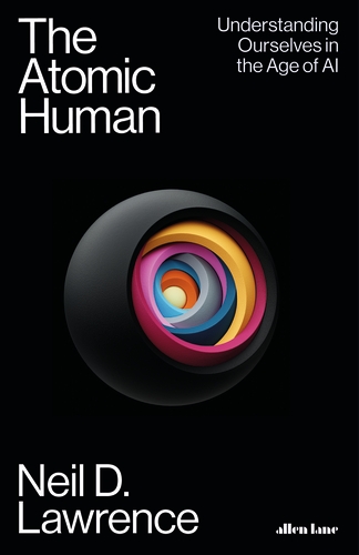
Figure: The Atomic Human (Lawrence, 2024).
Information and Embodiment
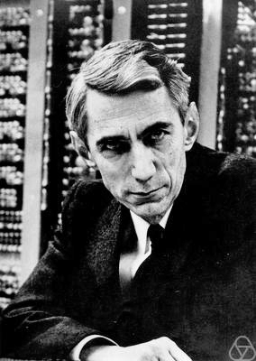
Figure: Claude Shannon (1916-2001)
| bits/min | billions | 2,000 |
| billion calculations/s | ~100 | a billion |
| embodiment | 20 minutes | 5 billion years |
Figure: Embodiment factors are the ratio between our ability to compute and our ability to communicate. Relative to the machine we are also locked in. In the table we represent embodiment as the length of time it would take to communicate one second’s worth of computation. For computers it is a matter of minutes, but for a human, it is a matter of thousands of millions of years.
Shannon measured information in bits: one bit is the result of a fair coin toss. He estimated \(\sim 12\) bits per English word on average (Shannon, 1948), which with typical speaking rates gives \(\sim 10\)–\(60\) bits per second for human communication Lawrence (2024). Machines communicate orders of magnitude faster — the embodiment factor is the ratio between compute and that narrow channel.
Shannon measured information in bits. Human communication is slow relative to machines — the embodiment factor. Lecture 3 derives \(H\); today we only need the bit as a unit of uncertainty and of bandwidth.
Shannon gave the unit used for bandwidth and embodiment factors. The derivation of \(H\) and the statement \(S=kH\) are LO2 in lecture 3. The bandwidth gap is a bottleneck on sharing thought, not a second no-go paired with Boltzmann. Lecture 4 applies the same bit accounting to locked-in communication.
Entropy and the Boltzmann Distribution
Hydrodynamica
When Laplace spoke of the curve of a simple molecule of air, he may well have been thinking of Daniel Bernoulli (1700-1782). Daniel Bernoulli was one name in a prodigious family. His father and brother were both mathematicians. Daniel’s main work was known as Hydrodynamica.
Figure: Daniel Bernoulli’s Hydrodynamica published in 1738. It was one of the first works to use the idea of conservation of energy. It used Newton’s laws to predict the behaviour of gases.
Daniel Bernoulli described a kinetic theory of gases, but it wasn’t until 170 years later when these ideas were verified after Einstein had proposed a model of Brownian motion which was experimentally verified by Jean Baptiste Perrin.
Figure: Daniel Bernoulli’s chapter on the kinetic theory of gases, for a review on the context of this chapter see Mikhailov (n.d.). For 1738 this is extraordinary thinking. The notion of kinetic theory of gases wouldn’t become fully accepted in Physics until 1908 when a model of Einstein’s was verified by Jean Baptiste Perrin.
Entropy Billiards
Figure: Bernoulli’s simple kinetic models of gases assume that the molecules of air operate like billiard balls. The displayed entropy is the Shannon entropy of the observed velocity histogram (a coarse-grained proxy, not full thermodynamic entropy).
import numpy as npp = np.random.randn(10000, 1)
xlim = [-4, 4]
x = np.linspace(xlim[0], xlim[1], 200)
y = 1/np.sqrt(2*np.pi)*np.exp(-0.5*x*x)Another important figure for Cambridge was the first to derive the probability distribution that results from small balls banging together in this manner. In doing so, James Clerk Maxwell founded the field of statistical physics.
Figure: James Clerk Maxwell 1831-1879 Derived distribution of velocities of particles in an ideal gas (elastic fluid).
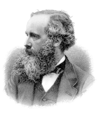
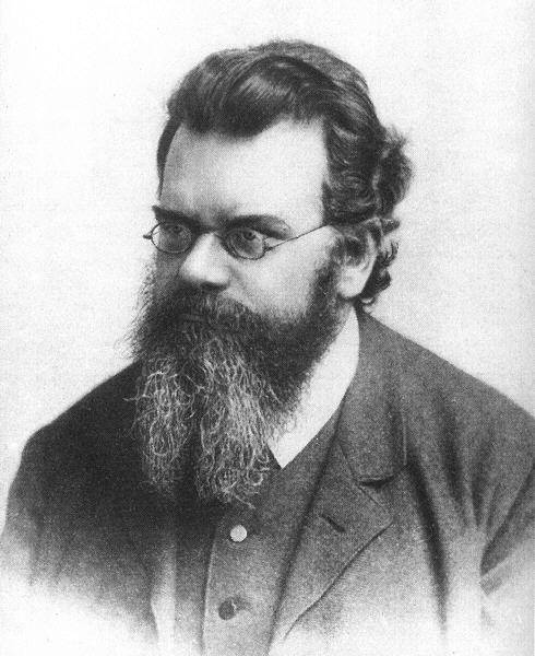
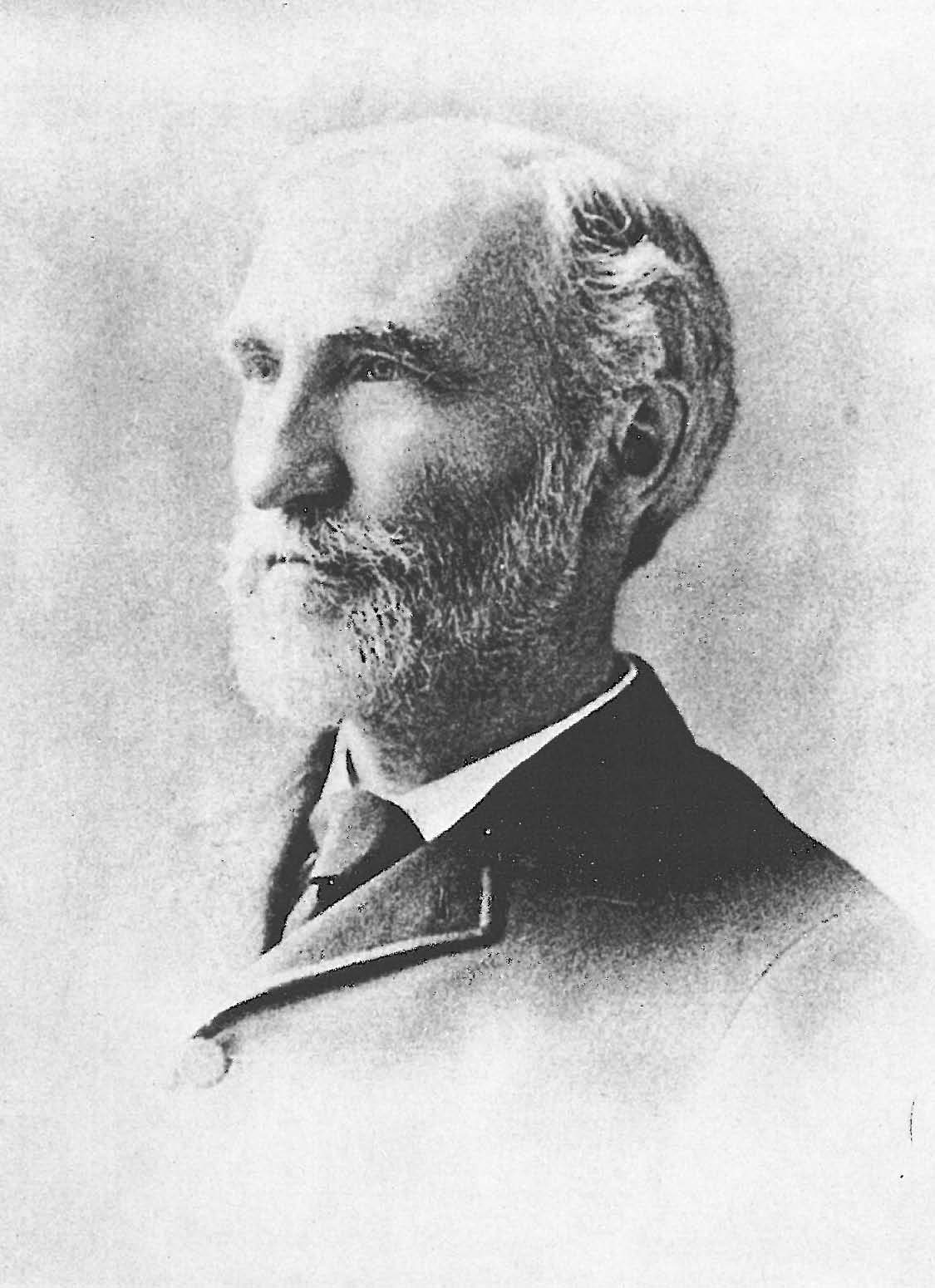
Figure: James Clerk Maxwell (1831-1879), Ludwig Boltzmann (1844-1906) Josiah Willard Gibbs (1839-1903)
Many of the ideas of early statistical physicists were rejected by a cadre of physicists who didn’t believe in the notion of a molecule. The stress of trying to have his ideas established caused Boltzmann to commit suicide in 1906, only two years before the same ideas became widely accepted.
Figure: Boltzmann’s paper Boltzmann (n.d.) which introduced the relationship between entropy and probability. A translation with notes is available in Sharp and Matschinsky (2015).
The important point about the uncertainty being represented here is that it is not genuine stochasticity, it is a lack of knowledge about the system. The techniques proposed by Maxwell, Boltzmann and Gibbs allow us to exactly represent the state of the system through a set of parameters that represent the sufficient statistics of the physical system. We know these values as the volume, temperature, and pressure. The challenge for us, when approximating the physical world with the techniques we will use is that we will have to sit somewhere between the deterministic and purely stochastic worlds that these different scientists described.
One ongoing characteristic of people who study probability and uncertainty is the confidence with which they hold opinions about it. Another leader of the Cavendish laboratory expressed his support of the second law of thermodynamics (which can be proven through the work of Gibbs/Boltzmann) with an emphatic statement at the beginning of his book.
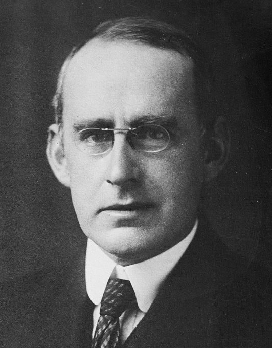
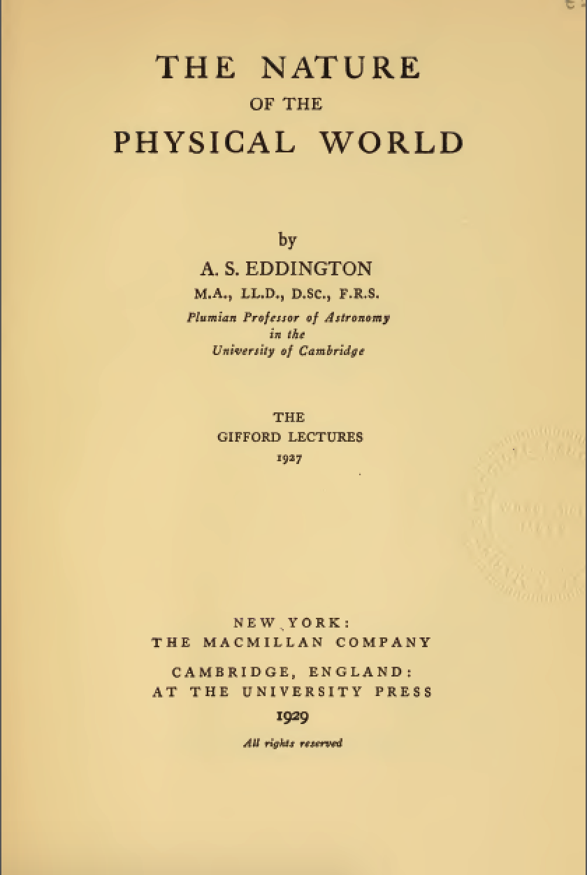
Figure: Eddington’s book on the Nature of the Physical World (Eddington, 1929)
The same Eddington is also famous for dismissing the ideas of a young Chandrasekhar who had come to Cambridge to study in the Cavendish lab. Chandrasekhar demonstrated the limit at which a star would collapse under its own weight to a singularity, but when he presented the work to Eddington, he was dismissive suggesting that there “must be some natural law that prevents this abomination from happening.”
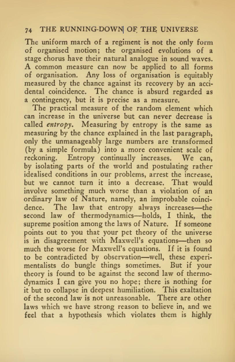
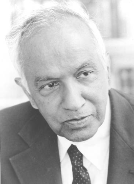
Figure: Chandrasekhar (1910-1995) derived the limit at which a star collapses in on itself. Eddington’s confidence in the 2nd law may have been what drove him to dismiss Chandrasekhar’s ideas, humiliating a young scientist who would later receive a Nobel prize for the work.
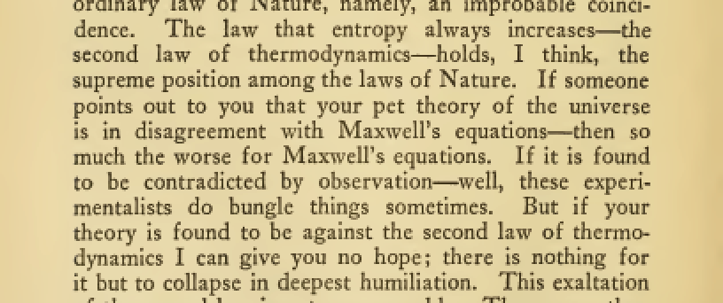
Figure: Eddington makes his feelings about the primacy of the second law clear. This primacy is perhaps because the second law can be demonstrated mathematically, building on the work of Maxwell, Gibbs and Boltzmann. Eddington (1929)
Presumably he meant that the creation of a black hole seemed to transgress the second law of thermodynamics, although later Hawking was able to show that blackholes do evaporate, but the time scales at which this evaporation occurs is many orders of magnitude slower than other processes in the universe.
Energy in Machine Learning
An energy in machine learning is a scalar score on a configuration: parameters, predictions, or binary states. Lower is preferred. An energy-based model turns that score into a distribution by the same exponential map used in statistical physics: \(p(x)\propto e^{-E(x)}\). Training often amounts to shaping \(E\) so that observed configurations sit in low-energy valleys. The examples below are familiar losses rewritten in that language — not new algorithms.
Under \(y_n=\mathbf{w}^\top\mathbf{x}_n+\varepsilon_n\) with \(\varepsilon_n\sim\mathscr{N}\left(0,\sigma^2\right)\), the negative log-likelihood is \(\frac{1}{2\sigma^2}E(\mathbf{w})\) plus constants. So ordinary least squares is maximum likelihood for a Gaussian or equivalently, minimising a quadratic energy.
When \(y\) is a one-hot label and \(\hat{y}\) a categorical prediction, cross-entropy is the energy of that pair. Softmax turns a vector of class energies (or logits) into a distribution. The functional \(-\log\hat{y}_c\) is the same one that appears in Shannon entropy \(\mathbb{E}[-\log P(y)]\), applied to a model distribution rather than the data distribution.
Ackley, Hinton and Sejnowski (Ackley et al., 1985) made the couplings \(W_{ij}\) learnable; Hopfield (Hopfield, 1982) used a similar pairwise energy for associative memory with fixed weights. When a Boltzmann or Gibbs occupation is written \(p\propto e^{-\beta E}\), the symbol \(E\) is the same kind of object minimised in regression and classification — a score over configurations, exponentiated into a distribution.
Boltzmann Seed
import numpy as npdef boltzmann(energies, beta):
"""Boltzmann probabilities $p_i \\propto e^{-\\beta E_i}$."""
log_w = -beta * np.asarray(energies, dtype=float)
log_w -= log_w.max()
w = np.exp(log_w)
return w / w.sum()
# Live check: boltzmann([0, 1], 1.0) -> about (0.731, 0.269)From Loss Landscapes to Hamiltonians
Seeing standard energies from machine learning as simply the logarithm of the probability leads to a form of static energy. It’s only the “potential energy” of a system. The aim is to find the minimum potential energy, and that is what we call learning. So what of “kinetic energy.”
We can think of the movement of the system as being the learning dynamics. The training is the movement of the parameters towards the minimum. That movement could have mass, and therefore momentum and kinetic energy.
Sometimes this analogy is proposed, like in momentum variables for stochastic gradient descent, but the analogy seems loose. One place where it’s tight is Hamiltonian Monte-Carlo.
Imagine a mass on a hill. It is sensitive to the pull of gravity as transmitted to it through the local slope. This is the potential energy, \(E(\mathbf{ w})\), acting as a force. The force is taken by the gradient of the potential energy which gives the slope, \(\nabla E(\mathbf{ w})\).
In gradient descent we take repeated steps opposite the gradient to reach a local minimum. We consider a little example below where the loss surface, the energy, is taken from a small regression problem where the true line has a gradient of \(m=1.4\) and an offset of \(c=-3.1\). We sample some data from that line by adding noise with a standard deviation of \(0.15\). Then we show the energy landscape for this system.
# Toy line: the error surface is the quadratic energy of the residual.
rng = np.random.default_rng(42)
x = np.linspace(0, 1, 25)
m_true, c_true = 1.4, -3.1
y = m_true * x + c_true + 0.15 * rng.standard_normal(x.shape)

m_vals = np.linspace(m_true - 3, m_true + 3, 80)
c_vals = np.linspace(c_true - 3, c_true + 3, 80)
m_grid, c_grid = np.meshgrid(m_vals, c_vals)
E_grid = np.zeros_like(m_grid)
for i in range(m_grid.shape[0]):
    for j in range(m_grid.shape[1]):
        E_grid[i, j] = ((y - m_grid[i, j] * x - c_grid[i, j]) ** 2).sum()

fig, ax = plt.subplots(figsize=(5, 5))
plot.regression_contour(fig, ax, m_vals, c_vals, E_grid)
mlai.write_figure('loss-energy-contour.svg', directory='./ml')
Figure: Contours of the least-squares energy \(E(m,c)=\sum_n(y_n-mx_n-c)^2\). Steepest descent walks toward the bowl.
In physics the parameters would be the position, \(q\), instead of the weights, \(w\). And typically (for a Hamiltonian) we denote the potential energy in physics by \(V(\cdot)\), so instead of \(E(\mathbf{ w})\) we have \(V(\mathbf{q})\).
So in mechanics, potential energy \(V(\mathbf{q})\) depends on position, \(q\). Gravity on a landscape is the everyday example mentioned above. But there are other forms of potential energy, for example the electrostatic energy of a charge configuration. Or the displacement of a spring. Gradient descent treats model parameters as a position \(\mathbf{q}\) and the training objective as \(V(\mathbf{q})\). The update \(\mathbf{q}\leftarrow\mathbf{q}-\eta\nabla V\) is a discrete, -dominated limit of a particle sliding on a potential. There is no inertia, there is only force from \(V(\cdot)\).
Modern neural network models train when the number of data points is very large. This makes computing the exact gradients very computationally expensive. The energy is typically decomposed as a sum over data points, \[ E(\mathbf{ w}, \mathbf{X}) = \sum_i E(\mathbf{ w}, \mathbf{x}_i) \] where the full data \(\mathbf{X} = \{ \mathbf{x}_i\}_{i=1}^n\).
So when \(n\) is huge, the sum becomes prophibitive. Stochastic gradient descent replaces \(\nabla V\) by an unbiased estimate from one example or a mini-batch. The walk is no longer smooth: the particle feels a jittering force. That is still dynamics on a potential; only the force estimate is random.
The closely related stochastic gradient with Langevin dynamics (SGLD, Welling and Teh (2011)) makes this connection very explicit. There the descent is taken to be a descent in a high friction regime which is subject to thermal noise. Thermal noise is the response of the descending particle to being bumped by particles of a surrounding fluid, like in Brownian motion. So SGLD is like Brownian motion in a potential well.
A classical particle has both potential and kinetic energy. Pure gradient descent never tracks a momentum conjugate to \(\mathbf{q}\); each step forgets velocity. Momentum SGD and Adam reintroduce inertia heuristically. Hamiltonian mechanics does it properly: introduce momentum \(\mathbf{p}\) and a kinetic energy \(T(\mathbf{p})\), usually \(\frac{1}{2}\mathbf{p}^\top M^{-1}\mathbf{p}\).
The Hamiltonian \(H\) is the sum of kinetic and potential energies. Hamilton’s equations are a mainstay of mechanics. They generate a flow on the joint \((\mathbf{q},\mathbf{p})\) space that conserves \(H\) when the system is isolated. For sampling, one chooses \(V(\mathbf{q})=-\log p(\mathbf{q})\) (up to a constant) so that the marginal on \(\mathbf{q}\) under the Boltzmann weight \(e^{-H}\) recovers the target density \(p(\mathbf{q})\).
Hamiltonian Monte Carlo (originally hybrid Monte Carlo) uses fictitious momentum variables so proposals move far in parameter space while staying near level sets of \(H\). Discretisation error is corrected by a Metropolis accept/reject on the Hamiltonian. The method turns gradient information about \(V\) into efficient exploration of high-dimensional densities. The method was originally developed for Bayesian sampling of neural network weights.
In these systems time is introduced as a “fictitious variable” representing the evolution of the algorithm and the momentum variables are known as “auxiliary variables.” The idea is to show that as time increases the system converges to the stationary distribution associated with the energy function, \(E(\mathbf{ w})\).
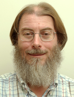
Figure: Radford M. Neal (University of Toronto).
Radford Neal is a Canadian computer scientist at the University of Toronto who (along with David MacKay) introduced ideas form Bayesian statistics into machine learning and neural networks. He introduced the hybrid Monte Varlo method for training neural networks with backpropagation (Neal, 1992). The Hamiltonian dynamics act as a proposal mechanism for posterior sampling over weights. His 1994 thesis (Neal, 1994) is still worth reading today. Alongside the benefits of the HMC approach he showed how infinite-width nets with suitable priors become Gaussian processes. Over time the term Hamiltonian was preferred to hybrid, and this allows us to really see the connection between “energy as loss” and “energy as the potential in a physical sampler.” Meaning that our sampling algorithm is being built by an analogy to a well-understood physical system.
Hamiltonian Monte Carlo Example
The reusable component lives in mlai.hmc. It has diagonal-mass kinetic energy, leapfrog proposals, and a Metropolis correction on \(\Delta H\). Below we first overlay leapfrog paths on a 2D quadratic potential (standard normal / least-squares bowl), then contrast an SGD point estimate with HMC samples for a small logistic regression — the same energy language as the lecture.
# 2D quadratic potential: V(q)=0.5||q||^2  (standard normal target).
# Leapfrog trajectories on the same contour language as regression_contour.
from mlai import HamiltonianMonteCarlo

potential = lambda q: 0.5 * np.dot(q, q)
grad_potential = lambda q: np.asarray(q, dtype=float)

hmc = HamiltonianMonteCarlo(
    potential=potential,
    grad_potential=grad_potential,
    step_size=0.15,
    n_steps=10,
)
result, trajectories = hmc.sample(
    q0=np.zeros(2), n_samples=40, random_state=0, return_trajectory=True
)

q1 = np.linspace(-3, 3, 80)
q2 = np.linspace(-3, 3, 80)
Q1, Q2 = np.meshgrid(q1, q2)
V_grid = 0.5 * (Q1 ** 2 + Q2 ** 2)

fig, ax = plt.subplots(figsize=(5, 5))
plot.hmc_contour_trajectories(
    ax, q1, q2, V_grid,
    trajectories=trajectories[:12],
    samples=result.samples,
    fontsize=16,
)
ax.set_title(f'HMC leapfrog paths (accept rate {result.accept_rate:.2f})')
mlai.write_figure('hmc-quadratic-trajectories.svg', directory='./ml')
Figure: Leapfrog trajectories and samples from teachable HMC on \(V(\mathbf{q})=\tfrac12\|\mathbf{q}\|^2\). Accept/reject keeps the chain on the Boltzmann target \(e^{-V}\).
# SGD point estimate vs HMC samples for logistic regression.
# Potential V(w) = -log p(w|D) with a flat prior (negative log-likelihood).
from mlai import LR, Basis, linear, HamiltonianMonteCarlo

rng = np.random.default_rng(0)
X = rng.normal(size=(60, 1))
y = (1.5 * X[:, 0] + 0.25 * rng.normal(size=60) > 0).astype(float).reshape(-1, 1)
model = LR(X, y, Basis(linear, number=2))

def potential(q):
    model.parameters = q
    return -float(model.log_likelihood())

def grad_potential(q):
    model.parameters = q
    return np.asarray(model.gradients, dtype=float)

# Point estimate by steepest descent on V
q_sgd = np.zeros(2)
for _ in range(250):
    q_sgd = q_sgd - 0.05 * grad_potential(q_sgd)

hmc = HamiltonianMonteCarlo(
    potential=potential, grad_potential=grad_potential,
    step_size=0.04, n_steps=10,
)
hmc_result = hmc.sample(q0=q_sgd, n_samples=300, random_state=1)

fig, axes = plt.subplots(3, 1, figsize=(6, 5), sharex=True)
plot.hmc_traces(axes, hmc_result, param_indices=[0, 1], fontsize=12)
axes[0].set_title(
    f'Logistic HMC traces (accept {hmc_result.accept_rate:.2f}); '
    f'SGD point = ({q_sgd[0]:.2f}, {q_sgd[1]:.2f})'
)
mlai.write_figure('hmc-logistic-traces.svg', directory='./ml')
print('SGD:', q_sgd, 'HMC mean:', hmc_result.samples.mean(axis=0))
Figure: Hamiltonian and weight traces for logistic regression. \(V(\mathbf{ w})=-\log p(\mathbf{ w}\mid\mathcal{D})\); SGD gives one downhill point, HMC a cloud of posterior samples.
Week 1 culmination: the energies named earlier are potentials. Descent is motion on \(V\); practice is stochastic; kinetic energy completes the Hamiltonian; HMC (Neal) is the sampler that uses both. The live demos use mlai.HamiltonianMonteCarlo: leapfrog paths on a quadratic potential, then logistic regression with an SGD point estimate versus an HMC posterior cloud.
Define This Week
After This Lecture
Worksheet 1: Socratic dialogue on Boltzmann / entropy / free energy before lecture 2. About ten turns; curiosity then skepticism; reflection. Use the template. Due 20 October, start of lecture 2. Quiz 1 in the first ten minutes of lecture 2 covers today’s probability and entropy review plus the seeds you should have pressed in the worksheet.
Further Reading
Probability distributions: Section 1.2 of Bishop (2006)
Chapter 1 of Lawrence (2024)
Boltzmann machines (optional colour) of Ackley et al. (1985)
Hopfield networks (optional colour) of Hopfield (1982)
Section 3.2.1 of Welling et al. (2026)
Section 11.4.2 of Welling et al. (2026)
Hybrid Monte Carlo for backpropagation networks of Neal (1992)
Bayesian Learning for Neural Networks (thesis) of Neal (1994)
Thanks!
For more information on these subjects and more you might want to check the following resources.
- company: Trent AI
- book: The Atomic Human
- twitter: @lawrennd
- podcast: The Talking Machines
- newspaper: Guardian Profile Page
- blog: http://inverseprobability.com
References
THat’s not strictly true because I can marginalise things I’m not interested in … but gives me a challenge of integrating over those variables which can lead to mathematical (or computational) headaches.↩︎
Fortunately, even if I’m totally wrong, the tools are widely deployed in a number of domains and your efforts in understanding them will bear fruit in one domain or another.↩︎