Introduction, Probability Review, and Motivation

Neil D. Lawrence

FW26, William Gates Building

This Session

  • Room FW26; eight Tuesdays from today
  • How worksheets and LLMs work (you are Socrates)
  • Probability and entropy review; energy in ML; then potential → Hamiltonian / HMC

Time Plan

Minutes Block
0–15 Course mechanics; questions list; the motivation and theme
15–35 ‘Socratic’ approach: curiosity, skepticism, submission rules
35–65 Probability review: product/sum/Bayes; basic distributions
65–75 Break
75–95 Entropy review (elementary \(H\)); bits and nats
95–110 Energy in ML; motivation and bandwidth; Boltzmann seed
110–118 Culmination: potential → stochastic → kinetic? → Hamiltonian / HMC
118–120 Worksheet 1 brief; Quiz 1 preview

Course Mechanics

  • Four Moodle quizzes (start of lectures 2, 5, 7, 8)
  • Four worksheets (W1: Socratic dialogue; later: notebook + reflection)
  • Marking is anonymous: candidate number, never name or CRSid on the file

Questions We Will Return To

  • Meet the questions today
  • Define later; interpret later still
  • Two of them only make sense after week 8

Information, energy and intelligence course notebook setup

Motivation

Perpetual Motion and Superintelligence

  • 1925: Motor vehicles (no perpetual motion)
  • 2025: Promises of superintelligence singularity
  • Same fundamental impossibility?

Why Perpetual Motion Failed

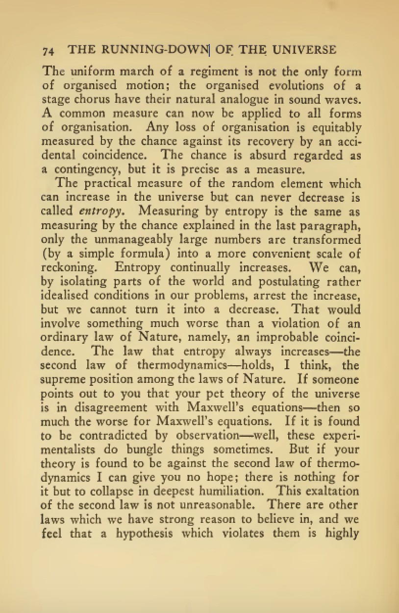
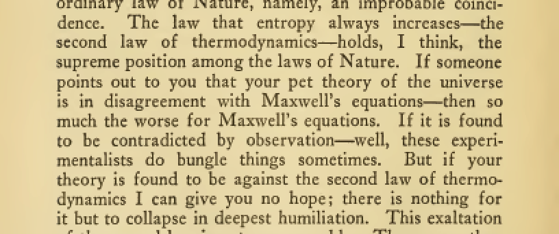
\[\frac{\text{d}H}{\text{d}t} \geq 0\]

  • Entropy always increases
  • No motion without entropy production
  • No work without energy input

An Equivalent Statement for Intelligence?

Maxwell’s Demon:

  • “Intelligent” entity that violates 2nd law
  • Resolution: Landauer’s principle?
  • Information erasure requires energy

Implication

  • Intelligence has thermodynamic cost
  • Information processing has physical limits

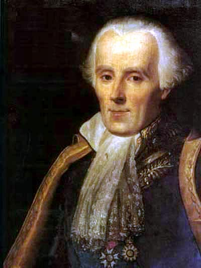
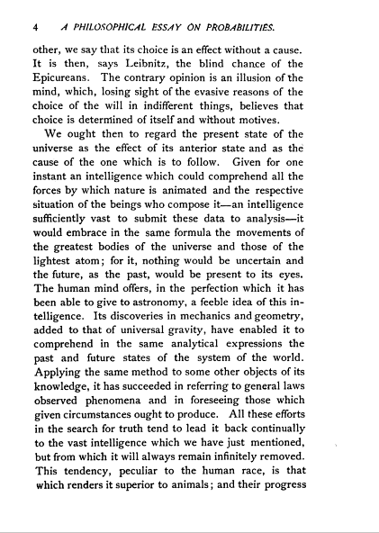
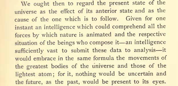
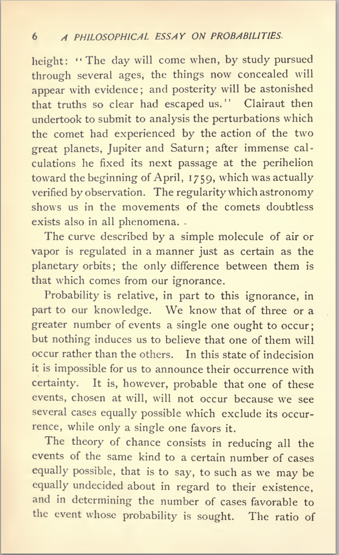
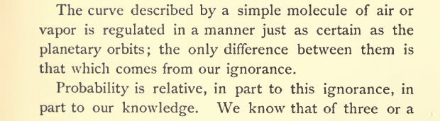
Laplace’s Gremlin

Laplace’s Gremlin

Philosophical Essay on Probabilities Laplace (1814) pg 5

Probability Review

  • Joint \(P(x,y)\): both
  • Marginal \(P(x)\): regardless of \(y\)
  • Conditional \(P(x\mid y)\): \(x\) given \(y\)

Product Rule and Sum Rule

  • Product: \(P(x,y)=P(x\mid y)P(y)\)
  • Sum: \(P(y)=\sum_x P(x,y)\)
  • Both are normalising bookkeeping, not modelling assumptions

Bayes’ Rule

\[ P(y\mid x)=\frac{P(x\mid y)P(y)}{P(x)} \]

  • Follows from the product rule and symmetry of the joint
  • Inverts the conditioning — updates a prior given a likelihood
  • \(P(x)=\sum_y P(x\mid y)P(y)\) when \(y\) is discrete

Bayes’ Theorem Example

  • There are two barrels in front of you. Barrel One contains 20 apples and 4 oranges. Barrel Two other contains 4 apples and 8 oranges. You choose a barrel randomly and select a fruit. It is an apple. What is the probability that the barrel was Barrel One?

Bayes’ Rule Example: Answer I

  • We are given: \[\begin{aligned} P(\text{F}=\text{A}|\text{B}=1) = & 20/24 \\ P(\text{F}=\text{A}|\text{B}=2) = & 4/12 \\ P(\text{B}=1) = & 0.5 \\ P(\text{B}=2) = & 0.5 \end{aligned}\]

Bayes’ Rule Example: Answer II

  • We use the sum rule to compute: \[\begin{aligned} P(\text{F}=\text{A}) = & P(\text{F}=\text{A}|\text{B}=1)P(\text{B}=1) \\& + P(\text{F}=\text{A}|\text{B}=2)P(\text{B}=2) \\ = & 20/24\times 0.5 + 4/12 \times 0.5 = 7/12 \end{aligned}\]
  • And Bayes’ rule tells us that: \[\begin{aligned} P(\text{B}=1|\text{F}=\text{A}) = & \frac{P(\text{F} = \text{A}|\text{B}=1)P(\text{B}=1)}{P(\text{F}=\text{A})}\\ = & \frac{20/24 \times 0.5}{7/12} = 5/7 \end{aligned}\]

Common Distributions

Named Distributions You Need

Five families recur across modelling. Know the support, the parameter, and one generative story for each.

Bernoulli and Binomial

  • Bernoulli(\(p\)): single binary trial; \(P(X=1)=p\)
  • Binomial(\(n,p\)): \(n\) i.i.d. Bernoulli trials; count of successes
  • Mean \(np\), variance \(np(1-p)\)

Poisson and Multinomial

  • Poisson(\(\lambda\)): counts in a fixed interval; mean \(=\) variance \(=\lambda\)
  • Multinomial(\(n,\mathbf{p}\)): \(n\) trials into \(K\) categories; generalises the binomial
  • Categories are exclusive; \(\sum_k p_k = 1\)

Poisson Distribution

  • Poisson distribution is used for ‘count data.’ For non-negative integers, \(y\), \[P(y) = \frac{\lambda^y}{y!}\exp(-\lambda)\]
  • Here \(\lambda\) is a rate parameter that can be thought of as the number of arrivals per unit time.
  • Poisson distributions can be used for disease count data. E.g. number of incidence of malaria in a district.

Poisson Distribution

Gaussian

  • \(\mathcal{N}(\mu,\sigma^2)\): continuous density on \(\mathbb{R}\)
  • Fixed by mean and variance; MaxEnt under those constraints
  • Multivariate form: mean vector and covariance matrix

The Gaussian Density

  • Perhaps the most common probability density.

\[\begin{align} p(y| \mu, \sigma^2) & = \frac{1}{\sqrt{2\pi\sigma^2}}\exp\left(-\frac{(y- \mu)^2}{2\sigma^2}\right)\\& \buildrel\triangle\over = \mathscr{N}\left(y|\mu,\sigma^2\right) \end{align}\]

Gaussian Density

Gaussian Density

\[ \mathscr{N}\left(y|\mu,\sigma^2\right) = \frac{1}{\sqrt{2\pi\sigma^2}} \exp\left(-\frac{(y-\mu)^2}{2\sigma^2}\right) \]

\(\sigma^2\) is the variance of the density and \(\mu\) is the mean.

Doubt

Worksheets and LLMs: Can you be Socrates?

Curiosity, Then Skepticism

Dialectical Vertigo

What you are describing, Skepticus, is a chronic but minor ailment of philosophers. It is called dialectical vertigo, and its cure is the immediate application of straightforward argumentation.

The Grasshopper to Skepticus in The Grassohopper: Games, Life and Utopia (Suits, 1978 pg 37)

Interacting with LLMs

  • Curiosity: open a question; let the model give a long answer (like Grasshopper)
  • Skepticism: take a claim and press it — “if that were true, then …” (like Skepticus)
  • Active thought is the point; the submitted transcript will be evidence of the probe

Worksheet Habit

  • Explore with as many models as you like
  • Submit one conversation of about ten prompt/answer turns
  • Early turns: open and curious; later turns: skeptical probes
  • Then a short reflection on what you learned
  • Template: assessments/handouts/ (dialogue + reflection)
  • Filename: candidatenumber_worksheet1_dialogue.md (and reflection)
  • Quiz 1 (next week) checks foundations you should have met here and in W1

Entropy Review

Computing Expectations Example

  • Consider the following distribution.
\(y\) 1 2 3 4
\(P\left(y\right)\) 0.3 0.2 0.1 0.4
  • What is the mean of the distribution?
  • What is the standard deviation of the distribution?
  • Are the mean and standard deviation representative of the distribution form?
  • What is the expected value of \(-\log P(y)\)?

Expectations Example: Answer

  • We are given:
\(y\) 1 2 3 4
\(P\left(y\right)\) 0.3 0.2 0.1 0.4
\(y^2\) 1 4 9 16
\(-\log(P(y))\) 1.204 1.609 2.302 0.916
  • Mean: \(1\times 0.3 + 2\times 0.2 + 3 \times 0.1 + 4 \times 0.4 = 2.6\)
  • Second moment: \(1 \times 0.3 + 4 \times 0.2 + 9 \times 0.1 + 16 \times 0.4 = 8.4\)
  • Variance: \(8.4 - 2.6\times 2.6 = 1.64\)
  • Standard deviation: \(\sqrt{1.64} = 1.2806\)

Expectations Example: Answer II

  • We are given that:
\(y\) 1 2 3 4
\(P\left(y\right)\) 0.3 0.2 0.1 0.4
\(y^2\) 1 4 9 16
\(-\log(P(y))\) 1.204 1.609 2.302 0.916
  • Expectation \(-\log(P(y))\): \(0.3\times 1.204 + 0.2\times 1.609 + 0.1\times 2.302 +0.4\times 0.916 = 1.280\)

Shannon entropy turns a distribution into a scalar measure of uncertainty.

  • Discrete: \(H(p) = -\sum_i p_i \log p_i\)
  • Base 2: bits; natural log: nats
  • Fair coin: \(H=1\) bit; certain outcome: \(H=0\)

Shannon’s definition is not yet …

  • … Clausius’s thermodynamic entropy (same formula, different motivation)
  • … a channel-capacity theorem

Entropy: physical and anthropomorphic

Joint, Conditional, Chain Rule (Names Only)

  • \(H(X,Y)\) joint uncertainty
  • \(H(X\mid Y)\) residual uncertainty after observing \(Y\)
  • Chain rule: \(H(X,Y)=H(X\mid Y) + H(Y)\)

Entropy and Probability

  • Entropy: no-go theorems
  • Probability: what we should do
  • Same \(H\), two jobs

Two Jobs

  • No-go: what is forbidden
  • Prescription: the \(p\) you should adopt
  • We will draw this idea out every week

Information and Embodiment
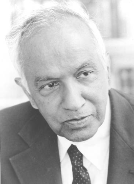
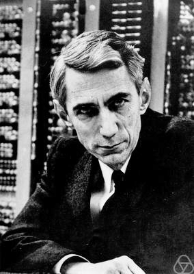
Claude Shannon

Embodiment Factors

bits/min billions 2,000
billion
calculations/s
~100 a billion
embodiment 20 minutes 5 billion years

Shannon Next Lecture

We are already counting in Shannon’s bits — embodiment is a communication bottleneck, not yet a theorem.

  • Lecture 3: why bits, and \(H=-\sum_i p_i\log p_i\) from axioms
  • Same functional form as Boltzmann \(S\); different operational reading
  • The intelligence question sharpens in lecture 4 (Landauer, Bauby)

Entropy and the Boltzmann Distribution

Hydrodynamica

Entropy Billiards

Velocity-bin entropy:

Energy in Machine Learning

In ML, an energy is a scalar assigned to a configuration: lower means preferred.

  • Losses are energies over parameters or predictions
  • Energy-based model: \(p(x)\propto e^{-E(x)}\) — same grammar as Boltzmann
  • Minimising \(E\) is the zero-temperature / MAP limit

\[ E(\mathbf{w})=\sum_n\left(y_n-\mathbf{w}^\top\mathbf{x}_n\right)^2 \]

  • Least squares = energy of the residual
  • Gaussian negative log-likelihood (up to additives and scale)
  • Gauss already linked this quadratic energy to the normal density

\[ E=-\sum_c y_c\log\hat{y}_c \]

  • Cross-entropy / log-loss scores the predictive distribution
  • Softmax: \(\hat{y}_c\propto e^{-E_c}\) — class scores as energies
  • Same arithmetic as \(\mathbb{E}[-\log p]\) (Shannon entropy of a model)

\[ E(\mathbf{s})=-\sum_i b_i s_i-\sum_{i<j}W_{ij}s_i s_j \]

  • Binary units \(s_i\in\{0,1\}\) or \(\{\pm 1\}\)
  • Biases plus pairwise couplings — classic BM has no triple terms
  • \(p(\mathbf{s})\propto e^{-E(\mathbf{s})/T}\): a learnable Gibbs distribution

Boltzmann Seed

A Prescription to Interrogate

For fixed mean energy \(U\), the maximum-entropy occupation is the Boltzmann distribution — same \(E\) grammar as the ML energies above.

  • \(p_i \propto e^{-\beta E_i}\) with coldness \(\beta = 1/kT\)
  • Normaliser \(Z=\sum_i e^{-\beta E_i}\), so \(p_i = e^{-\beta E_i}/Z\)
  • Week 2: name Gibbs, account with free energy \(F=U-TS\); Carnot–Clausius history

From Loss Landscapes to Hamiltonians

Gradient descent: ‘walking downhill’

  • Contours of \(E(\mathbf{ w})\) = elevation lines on a hill
  • Steepest descent: step opposite \(\nabla E\)
  • Same \(E\) as least squares / negative log-likelihood

The loss is a potential energy \(V(\mathbf{q})\) on parameter space.

  • Configuration \(\mathbf{q}=\mathbf{ w}\): where the system sits
  • Force \(\propto -\nabla V\): direction of steepest descent
  • Common analogy: ball in a bowl; GD is the overdamped limit

SGD estimates \(\nabla V\) from a random mini-batch

  • Full-batch \(\nabla V\): exact force, expensive
  • SGD: noisy force; cheap; enables online updates
  • Noise can help escape shallow traps (less relevant for convex bowls)

Where is the kinetic energy?

  • GD / SGD: overdamped—friction, no momentum inventory
  • Momentum methods (heavy ball, Adam): heuristic inertia
  • Physics: kinetic energy \(T(\mathbf{p})\) lives on momentum \(\mathbf{p}\)

\[ H(\mathbf{q},\mathbf{p}) = T(\mathbf{p}) + V(\mathbf{q}) \]

  • Total energy = kinetic + potential
  • Hamilton: \(\dot{\mathbf{q}}=\partial H/\partial\mathbf{p}\), \(\dot{\mathbf{p}}=-\partial H/\partial\mathbf{q}\)
  • \(H\) conserved along the flow (ideal, frictionless case)

HMC: invent momentum, simulate Hamiltonian dynamics, accept/reject.

  • Draw \(\mathbf{p}\sim\mathcal{N}(0,M)\); simulate leapfrog steps on \(H\)
  • Propose \((\mathbf{q}',\mathbf{p}')\); Metropolis test on \(H\)
  • Marginal samples of \(\mathbf{q}\) target \(p(\mathbf{q})\propto e^{-V(\mathbf{q})}\)
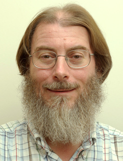
Radford Neal brought Hamiltonian Monte Carlo into Bayesian neural nets.

  • Toronto; Bayesian learning and MCMC
  • Hybrid Monte Carlo for backpropagation networks (Neal, 1992)
  • PhD thesis: Bayesian neural nets; infinite width \(\to\) GP (Neal, 1994)

Hamiltonian Monte Carlo Example

  • Target: \(V(\mathbf{q})=-\log p(\mathbf{q}\mid\mathcal{D})\) (loss as potential)
  • HamiltonianMonteCarlo in mlai; trace \(H\) and accept rate
  • Contrast: SGD point estimate vs HMC posterior samples

Define This Week

  • Product rule, sum rule, Bayes
  • Bernoulli, binomial, Poisson, multinomial, Gaussian
  • \(H=-\sum_i p_i\log p_i\) (bits or nats)
  • Energy scores: quadratic, cross-entropy, BM pairwise
  • Loss landscape as potential \(V\); ask for kinetic \(K\); Hamiltonian \(H=K+V\)
  • Seed: \(p_i = e^{-\beta E_i}/Z\); HMC via mlai (Neal)

After This Lecture

  • Worksheet 1 released; due 20 October (Socratic dialogue)
  • Quiz 1 next week: probability, entropy, Week 1 seeds

Further Reading

  • Probability distributions: Section 1.2 of Bishop (2006)

  • Chapter 1 of Lawrence (2024)

  • Boltzmann machines (optional colour) of Ackley et al. (1985)

  • Hopfield networks (optional colour) of Hopfield (1982)

  • Section 3.2.1 of Welling et al. (2026)

  • Section 11.4.2 of Welling et al. (2026)

  • Hybrid Monte Carlo for backpropagation networks of Neal (1992)

  • Bayesian Learning for Neural Networks (thesis) of Neal (1994)

Thanks!

References

Ackley, D., Hinton, G.E., Sejnowski, T.J., 1985. A learning algorithm for Boltzmann machines. Cognitive Science 9, 147–169.
Bishop, C.M., 2006. Pattern recognition and machine learning. springer.
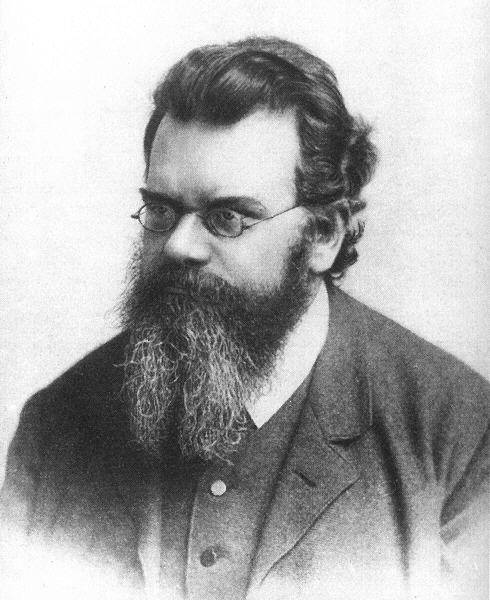
Boltzmann, L., n.d. Über die Beziehung zwischen dem zweiten Hauptsatze der mechanischen Warmetheorie und der Wahrscheinlichkeitsrechnung, respective den Sätzen über das wärmegleichgewicht. Sitzungberichte der Kaiserlichen Akademie der Wissenschaften. Mathematisch-Naturwissen Classe. Abt. II LXXVI, 373–435.
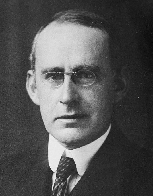
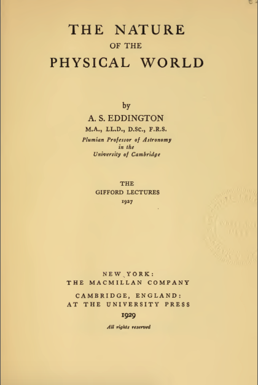
Eddington, A.S., 1929. The nature of the physical world. Dent (London). https://doi.org/10.2307/2180099
Hopfield, J.J., 1982. Neural networks and physical systems with emergent collective computational abilities. Proceedings of the National Academy of Sciences 79, 2554–2558.
Laplace, P.S., 1814. Essai philosophique sur les probabilités, 2nd ed. Courcier, Paris.
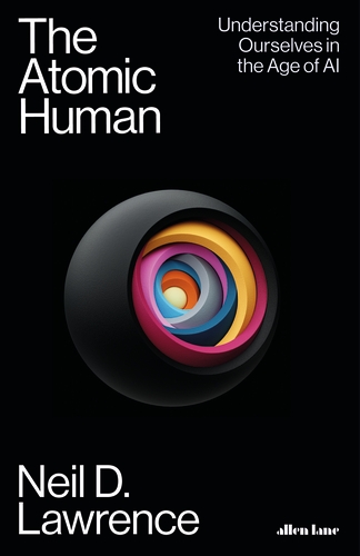
Lawrence, N.D., 2024. The atomic human: Understanding ourselves in the age of AI. Allen Lane.
Mikhailov, G.K., n.d. Daniel bernoulli, hydrodynamica (1738).
Neal, R.M., 1994. Bayesian learning for neural networks (PhD thesis). Dept. of Computer Science, University of Toronto.
Neal, R.M., 1992. Bayesian training of backpropagation networks by the hybrid Monte Carlo method (No. CRG-TR-92-1). Department of Computer Science, University of Toronto, Canada.
Sharp, K., Matschinsky, F., 2015. Translation of Ludwig Boltzmann’s paper “on the relationship between the second fundamental theorem of the mechanical theory of heat and probability calculations regarding the conditions for thermal equilibrium.” Entropy 17, 1971–2009. https://doi.org/10.3390/e17041971
Suits, B., 1978. The grasshopper: Games, life and utopia. University of Toronto Press, Toronto.
Welling, M., Lu, S., Holdijk, L., 2026. Generative AI and stochastic thermodynamics: A tale of free energies. Cambridge University Press, Cambridge, U.K.