Week 4: The Challenges of Data Science

[reveal]

Neil D. Lawrence

Abstract:

In the first lecture, we laid out the underpinning phenomena that give us the landscape of data science. In this lecture we unpick the challenges that landscape presents us with. The material gives you context for why data science is very different from standard software engineering, and how data science problems need to be approached including the many different aspects that need to be considered. We will look at the challenges of deploying data science solutions in practice. We categorize them into three groups.

Introduction

Data science is an emerging discipline. That makes it harder to make clean decisions about what any given individual will need to know to become a data scientist. Those of you who are studying now will be those that define the discipline. As we deploy more data driven decision making in the world, the role will be refined. Until we achieve that refinement, your knowledge needs to be broad based.

In this lecture we will first continue our theme of how our limitations as humans mean that our analysis of data can be affected, and I will introduce an analogy that should help you understand how data science differs significantly from traditional software engineering.

Data Science as Debugging

One challenge for existing information technology professionals is realizing the extent to which a software ecosystem based on data differs from a classical ecosystem. In particular, by ingesting data we bring unknowns/uncontrollables into our decision-making system. This presents opportunity for adversarial exploitation and unforeseen operation.

blog post on Data Science as Debugging.

Starting with the analysis of a data set, the nature of data science is somewhat difference from classical software engineering.

One analogy I find helpful for understanding the depth of change we need is the following. Imagine as a software engineer, you find a USB stick on the ground. And for some reason you know that on that USB stick is a particular API call that will enable you to make a significant positive difference on a business problem. You don’t know which of the many library functions on the USB stick are the ones that will help. And it could be that some of those library functions will hinder, perhaps because they are just inappropriate or perhaps because they have been placed there maliciously. The most secure thing to do would be to not introduce this code into your production system at all. But what if your manager told you to do so, how would you go about incorporating this code base?

The answer is very carefully. You would have to engage in a process more akin to debugging than regular software engineering. As you understood the code base, for your work to be reproducible, you should be documenting it, not just what you discovered, but how you discovered it. In the end, you typically find a single API call that is the one that most benefits your system. But more thought has been placed into this line of code than any line of code you have written before.

An enormous amount of debugging would be required. As the nature of the code base is understood, software tests to verify it also need to be constructed. At the end of all your work, the lines of software you write to interact with the software on the USB stick are likely to be minimal. But more thought would be put into those lines than perhaps any other lines of code in the system.

Even then, when your API code is introduced into your production system, it needs to be deployed in an environment that monitors it. We cannot rely on an individual’s decision making to ensure the quality of all our systems. We need to create an environment that includes quality controls, checks, and bounds, tests, all designed to ensure that assumptions made about this foreign code base are remaining valid.

This situation is akin to what we are doing when we incorporate data in our production systems. When we are consuming data from others, we cannot assume that it has been produced in alignment with our goals for our own systems. Worst case, it may have been adversarially produced. A further challenge is that data is dynamic. So, in effect, the code on the USB stick is evolving over time.

It might see that this process is easy to formalize now, we simply need to check what the formal software engineering process is for debugging, because that is the current software engineering activity that data science is closest to. But when we look for a formalization of debugging, we find that there is none. Indeed, modern software engineering mainly focusses on ensuring that code is written without bugs in the first place.

Lessons

1. When you begin an analysis, behave as a debugger.

• Write test code as you go. Document those tests and ensure they are accessible by others.
• Understand the landscape of your data. Be prepared to try several different approaches to the data set.
• Be constantly skeptical.
• Use the best tools available, develop a deep understand how they work.
• Share your experience of what challenges you’re facing. Have others (software engineers, fellow data analysts, your manager) review your work.
• Never go straight for the goal: you’d never try and write the API call straight away on the discarded hard drive, so why are you launching your classification algorithm before visualizing the data?
• Ensure your analysis is documented and accessible. If your code does go wrong in production, you’ll need to be able to retrace to where the error crept in.

2. When managing the data science process, don’t treat it as standard code development.

• Don’t deploy a traditional agile development pipeline and expect it to work the same way it does for standard code development. Think about how you handle bugs, think about how you would handle very many bugs.
• Don’t leave the data scientist alone to wade through the mess.
• Integrate the data analysis with your other team activities. Have the software engineers and domain experts work closely with the data scientists. This is vital for providing the data scientists with the technical support they need, but also managing the expectations of the engineers in terms of when and how the data will be able to deliver.

Recommendation: Anecdotally, resolving a machine learning challenge requires 80% of the resource to be focused on the data and perhaps 20% to be focused on the model. But many companies are too keen to employ machine learning engineers who focus on the models, not the data. We should change our hiring priorities and training. Universities cannot provide the understanding of how to data-wrangle. Companies must fill this gap.

Statistics to Deep Learning

What is Machine Learning?

Machine learning allows us to extract knowledge from data to form a prediction.

\[\text{data} + \text{model} \stackrel{\text{compute}}{\rightarrow} \text{prediction}\]

A machine learning prediction is made by combining a model with data to form the prediction. The manner in which this is done gives us the machine learning algorithm.

Machine learning models are mathematical models which make weak assumptions about data, e.g. smoothness assumptions. By combining these assumptions with the data, we observe we can interpolate between data points or, occasionally, extrapolate into the future.

Machine learning is a technology which strongly overlaps with the methodology of statistics. From a historical/philosophical view point, machine learning differs from statistics in that the focus in the machine learning community has been primarily on accuracy of prediction, whereas the focus in statistics is typically on the interpretability of a model and/or validating a hypothesis through data collection.

The rapid increase in the availability of compute and data has led to the increased prominence of machine learning. This prominence is surfacing in two different but overlapping domains: data science and artificial intelligence.

From Model to Decision

The real challenge, however, is end-to-end decision making. Taking information from the environment and using it to drive decision making to achieve goals.

Classical Statistical Analysis

Despite the shift of emphasis, traditional statistical techniques are more important than ever. One of the few ways we have to validate the analyses we create is to make use of visualizations, randomized testing and other forms of statistical analysis. You will have explored some of these ideas in earlier courses in machine learning. In this unit we provide some review material in a practical sheet to bring some of those ideas together in the context of data science.

What is Machine Learning?

What is machine learning? At its most basic level machine learning is a combination of

\[\text{data} + \text{model} \stackrel{\text{compute}}{\rightarrow} \text{prediction}\]

where data is our observations. They can be actively or passively acquired (meta-data). The model contains our assumptions, based on previous experience. That experience can be other data, it can come from transfer learning, or it can merely be our beliefs about the regularities of the universe. In humans our models include our inductive biases. The prediction is an action to be taken or a categorization or a quality score. The reason that machine learning has become a mainstay of artificial intelligence is the importance of predictions in artificial intelligence. The data and the model are combined through computation.

In practice we normally perform machine learning using two functions. To combine data with a model we typically make use of:

a prediction function it is used to make the predictions. It includes our beliefs about the regularities of the universe, our assumptions about how the world works, e.g., smoothness, spatial similarities, temporal similarities.

an objective function it defines the ‘cost’ of misprediction. Typically, it includes knowledge about the world’s generating processes (probabilistic objectives) or the costs we pay for mispredictions (empirical risk minimization).

The combination of data and model through the prediction function and the objective function leads to a learning algorithm. The class of prediction functions and objective functions we can make use of is restricted by the algorithms they lead to. If the prediction function or the objective function are too complex, then it can be difficult to find an appropriate learning algorithm. Much of the academic field of machine learning is the quest for new learning algorithms that allow us to bring different types of models and data together.

A useful reference for state of the art in machine learning is the UK Royal Society Report, Machine Learning: Power and Promise of Computers that Learn by Example.

You can also check my post blog post on What is Machine Learning?.

Artificial Intelligence and Data Science

Machine learning technologies have been the driver of two related, but distinct disciplines. The first is data science. Data science is an emerging field that arises from the fact that we now collect so much data by happenstance, rather than by experimental design. Classical statistics is the science of drawing conclusions from data, and to do so statistical experiments are carefully designed. In the modern era we collect so much data that there’s a desire to draw inferences directly from the data.

As well as machine learning, the field of data science draws from statistics, cloud computing, data storage (e.g. streaming data), visualization and data mining.

In contrast, artificial intelligence technologies typically focus on emulating some form of human behaviour, such as understanding an image, or some speech, or translating text from one form to another. The recent advances in artificial intelligence have come from machine learning providing the automation. But in contrast to data science, in artificial intelligence the data is normally collected with the specific task in mind. In this sense it has strong relations to classical statistics.

Classically artificial intelligence worried more about logic and planning and focused less on data driven decision making. Modern machine learning owes more to the field of Cybernetics (Wiener, 1948) than artificial intelligence. Related fields include robotics, speech recognition, language understanding and computer vision.

There are strong overlaps between the fields, the wide availability of data by happenstance makes it easier to collect data for designing AI systems. These relations are coming through wide availability of sensing technologies that are interconnected by cellular networks, WiFi and the internet. This phenomenon is sometimes known as the Internet of Things, but this feels like a dangerous misnomer. We must never forget that we are interconnecting people, not things.

What does Machine Learning do?

Any process of automation allows us to scale what we do by codifying a process in some way that makes it efficient and repeatable. Machine learning automates by emulating human (or other actions) found in data. Machine learning codifies in the form of a mathematical function that is learnt by a computer. If we can create these mathematical functions in ways in which they can interconnect, then we can also build systems.

Machine learning works through codifying a prediction of interest into a mathematical function. For example, we can try and predict the probability that a customer wants to by a jersey given knowledge of their age, and the latitude where they live. The technique known as logistic regression estimates the odds that someone will by a jumper as a linear weighted sum of the features of interest.

\[ \text{odds} = \frac{p(\text{bought})}{p(\text{not bought})} \]

\[ \log \text{odds} = w_0 + w_1 \text{age} + w_2 \text{latitude}.\] Here \(w_0\), \(w_1\) and \(w_2\) are the parameters of the model. If \(w_1\) and \(w_2\) are both positive, then the log-odds that someone will buy a jumper increase with increasing latitude and age, so the further north you are and the older you are the more likely you are to buy a jumper. The parameter \(w_0\) is an offset parameter and gives the log-odds of buying a jumper at zero age and on the equator. It is likely to be negative¹ indicating that the purchase is odds-against. This is also a classical statistical model, and models like logistic regression are widely used to estimate probabilities from ad-click prediction to disease risk.

This is called a generalized linear model, we can also think of it as estimating the probability of a purchase as a nonlinear function of the features (age, latitude) and the parameters (the \(w\) values). The function is known as the sigmoid or logistic function, thus the name logistic regression.

Sigmoid Function

Figure: The logistic function.

The function has this characeristic ‘s’-shape (from where the term sigmoid, as in sigma, comes from). It also takes the input from the entire real line and ‘squashes’ it into an output that is between zero and one. For this reason it is sometimes also called a ‘squashing function’.

The sigmoid comes from the inverting the odds ratio, \[ \frac{\pi}{(1-\pi)} \] where \(\pi\) is the probability of a positive outcome and \(1-\pi\) is the probability of a negative outcome

\[ p(\text{bought}) = \sigma\left(w_0 + w_1 \text{age} + w_2 \text{latitude}\right).\]

In the case where we have features to help us predict, we sometimes denote such features as a vector, \(\mathbf{ x}\), and we then use an inner product between the features and the parameters, \(\mathbf{ w}^\top \mathbf{ x}= w_1 x_1 + w_2 x_2 + w_3 x_3 ...\), to represent the argument of the sigmoid.

\[ p(\text{bought}) = \sigma\left(\mathbf{ w}^\top \mathbf{ x}\right).\] More generally, we aim to predict some aspect of our data, \(y\), by relating it through a mathematical function, \(f(\cdot)\), to the parameters, \(\mathbf{ w}\) and the data, \(\mathbf{ x}\).

\[ y= f\left(\mathbf{ x}, \mathbf{ w}\right).\] We call \(f(\cdot)\) the prediction function.

To obtain the fit to data, we use a separate function called the objective function that gives us a mathematical representation of the difference between our predictions and the real data.

\[E(\mathbf{ w}, \mathbf{Y}, \mathbf{X})\] A commonly used examples (for example in a regression problem) is least squares, \[E(\mathbf{ w}, \mathbf{Y}, \mathbf{X}) = \sum_{i=1}^n\left(y_i - f(\mathbf{ x}_i, \mathbf{ w})\right)^2.\]

If a linear prediction function is combined with the least squares objective function, then that gives us a classical linear regression, another classical statistical model. Statistics often focusses on linear models because it makes interpretation of the model easier. Interpretation is key in statistics because the aim is normally to validate questions by analysis of data. Machine learning has typically focused more on the prediction function itself and worried less about the interpretation of parameters. In statistics, where interpretation is typically more important than prediction, parameters are normally denoted by \(\boldsymbol{\beta}\) instead of \(\mathbf{ w}\).

A key difference between statistics and machine learning, is that (traditionally) machine learning has focussed on predictive capability and statistics has focussed on interpretability. That means that in a statistics class far more emphasis will be placed on interpretation of the parameters. In machine learning, the parameters, $, are just a means to an end. But in statistics, when we denote the parameters by \(\boldsymbol{\beta}\), we often use the parameters to tell us something about the disease.

So we move between \[ p(\text{bought}) = \sigma\left(w_0 + w_1 \text{age} + w_2 \text{latitude}\right).\]

to denote the emphasis is on predictive power to

\[ p(\text{bought}) = \sigma\left(\beta_0 + \beta_1 \text{age} + \beta_2 \text{latitude}\right).\]

to denote the emphasis is on interpretation of the parameters.

Another effect of the focus on prediction in machine learning is that non-linear approaches, which can be harder to interpret, are more widely deployedin machine learning – they tend to improve quality of predictions at the expense of interpretability.

Logistic Regression

A logistic regression is an approach to classification which extends the linear basis function models we’ve already explored. Rather than modeling the output of the function directly the assumption is that we model the log-odds with the basis functions.

The odds are defined as the ratio of the probability of a positive outcome, to the probability of a negative outcome. If the probability of a positive outcome is denoted by \(\pi\), then the odds are computed as \(\frac{\pi}{1-\pi}\). Odds are widely used by bookmakers in gambling, although a bookmakers odds won’t normalise: i.e. if you look at the equivalent probabilities, and sum over the probability of all outcomes the bookmakers are considering, then you won’t get one. This is how the bookmaker makes a profit. Because a probability is always between zero and one, the odds are always between \(0\) and \(\infty\). If the positive outcome is unlikely the odds are close to zero, if it is very likely then the odds become close to infinite. Taking the logarithm of the odds maps the odds from the positive half space to being across the entire real line. Odds that were between 0 and 1 (where the negative outcome was more likely) are mapped to the range between \(-\infty\) and \(0\). Odds that are greater than 1 are mapped to the range between \(0\) and \(\infty\). Considering the log odds therefore takes a number between 0 and 1 (the probability of positive outcome) and maps it to the entire real line. The function that does this is known as the logit function, \(g^{-1}(p_i) = \log\frac{p_i}{1-p_i}\). This function is known as a link function.

For a standard regression we take, \[ f(\mathbf{ x}) = \mathbf{ w}^\top \boldsymbol{ \phi}(\mathbf{ x}), \] if we want to perform classification we perform a logistic regression. \[ \log \frac{\pi}{(1-\pi)} = \mathbf{ w}^\top \boldsymbol{ \phi}(\mathbf{ x}) \] where the odds ratio between the positive class and the negative class is given by \[ \frac{\pi}{(1-\pi)} \] The odds can never be negative, but can take any value from 0 to \(\infty\). We have defined the link function as taking the form \(g^{-1}(\cdot)\) implying that the inverse link function is given by \(g(\cdot)\). Since we have defined, \[ g^{-1}(\pi) = \mathbf{ w}^\top \boldsymbol{ \phi}(\mathbf{ x}) \] we can write \(\pi\) in terms of the inverse link function, \(g(\cdot)\) as \[ \pi = g(\mathbf{ w}^\top \boldsymbol{ \phi}(\mathbf{ x})). \]

Basis Function

We’ll define our prediction, objective and gradient functions below. But before we start, we need to define a basis function for our model. Let’s start with the linear basis.

import numpy as np

import mlai

from mlai import linear

Prediction Function

Now we have the basis function let’s define the prediction function.

import numpy as np

def predict(w, x, basis=linear, **kwargs):
    "Generates the prediction function and the basis matrix."
    Phi = basis(x, **kwargs)
    f = np.dot(Phi, w)
    return 1./(1+np.exp(-f)), Phi

This inverse of the link function is known as the logistic (thus the name logistic regression) or sometimes it is called the sigmoid function. For a particular value of the input to the link function, \(f_i = \mathbf{ w}^\top \boldsymbol{ \phi}(\mathbf{ x}_i)\) we can plot the value of the inverse link function as below.

By replacing the inverse link with the sigmoid we can write \(\pi\) as a function of the input and the parameter vector as, \[ \pi(\mathbf{ x},\mathbf{ w}) = \frac{1}{1+\exp\left(-\mathbf{ w}^\top \boldsymbol{ \phi}(\mathbf{ x})\right)}. \] The process for logistic regression is as follows. Compute the output of a standard linear basis function composition (\(\mathbf{ w}^\top \boldsymbol{ \phi}(\mathbf{ x})\), as we did for linear regression) and then apply the inverse link function, \(g(\mathbf{ w}^\top \boldsymbol{ \phi}(\mathbf{ x}))\). In logistic regression this involves squashing it with the logistic (or sigmoid) function. Use this value, which now has an interpretation as a probability in a Bernoulli distribution to form the likelihood. Then we can assume conditional independence of each data point given the parameters and develop a likelihod for the entire data set.

As we discussed last time, the Bernoulli likelihood is of the form, \[ P(y_i|\mathbf{ w}, \mathbf{ x}) = \pi_i^{y_i} (1-\pi_i)^{1-y_i} \] which we can think of as clever trick for mathematically switching between two probabilities if we were to write it as code it would be better described as

def bernoulli(x, y, pi):
    if y == 1:
        return pi(x)
    else:
        return 1-pi(x)

but writing it mathematically makes it easier to write our objective function within a single mathematical equation.

Maximum Likelihood

To obtain the parameters of the model, we need to maximize the likelihood, or minimize the objective function, normally taken to be the negative log likelihood. With a data conditional independence assumption the likelihood has the form, \[ P(\mathbf{ y}|\mathbf{ w}, \mathbf{X}) = \prod_{i=1}^nP(y_i|\mathbf{ w}, \mathbf{ x}_i). \] which can be written as a log likelihood in the form \[ \log P(\mathbf{ y}|\mathbf{ w}, \mathbf{X}) = \sum_{i=1}^n\log P(y_i|\mathbf{ w}, \mathbf{ x}_i) = \sum_{i=1}^n y_i \log \pi_i + \sum_{i=1}^n(1-y_i)\log (1-\pi_i) \] and if we take the probability of positive outcome for the \(i\)th data point to be given by \[ \pi_i = g\left(\mathbf{ w}^\top \boldsymbol{ \phi}(\mathbf{ x}_i)\right), \] where \(g(\cdot)\) is the inverse link function, then this leads to an objective function of the form, \[ E(\mathbf{ w}) = - \sum_{i=1}^ny_i \log g\left(\mathbf{ w}^\top \boldsymbol{ \phi}(\mathbf{ x}_i)\right) - \sum_{i=1}^n(1-y_i)\log \left(1-g\left(\mathbf{ w}^\top \boldsymbol{ \phi}(\mathbf{ x}_i)\right)\right). \]

import numpy as np

def objective(g, y):
    "Computes the objective function."
    labs = np.asarray(y, dtype=float).flatten()
    posind = np.where(labs==1)
    negind = np.where(labs==0)
    return -np.log(g[posind, :]).sum() - np.log(1-g[negind, :]).sum()

As normal, we would like to minimize this objective. This can be done by differentiating with respect to the parameters of our prediction function, \(\pi(\mathbf{ x};\mathbf{ w})\), for optimisation. The gradient of the likelihood with respect to \(\pi(\mathbf{ x};\mathbf{ w})\) is of the form, \[ \frac{\text{d}E(\mathbf{ w})}{\text{d}\mathbf{ w}} = -\sum_{i=1}^n \frac{y_i}{g\left(\mathbf{ w}^\top \boldsymbol{ \phi}(\mathbf{ x})\right)}\frac{\text{d}g(f_i)}{\text{d}f_i} \boldsymbol{ \phi}(\mathbf{ x}_i) + \sum_{i=1}^n \frac{1-y_i}{1-g\left(\mathbf{ w}^\top \boldsymbol{ \phi}(\mathbf{ x})\right)}\frac{\text{d}g(f_i)}{\text{d}f_i} \boldsymbol{ \phi}(\mathbf{ x}_i) \] where we used the chain rule to develop the derivative in terms of \(\frac{\text{d}g(f_i)}{\text{d}f_i}\), which is the gradient of the inverse link function (in our case the gradient of the sigmoid function).

So the objective function now depends on the gradient of the inverse link function, as well as the likelihood depends on the gradient of the inverse link function, as well as the gradient of the log likelihood, and naturally the gradient of the argument of the inverse link function with respect to the parameters, which is simply \(\boldsymbol{ \phi}(\mathbf{ x}_i)\).

The only missing term is the gradient of the inverse link function. For the sigmoid squashing function we have, \[\begin{align*} g(f_i) &= \frac{1}{1+\exp(-f_i)}\\ &=(1+\exp(-f_i))^{-1} \end{align*}\] and the gradient can be computed as \[\begin{align*} \frac{\text{d}g(f_i)}{\text{d} f_i} & = \exp(-f_i)(1+\exp(-f_i))^{-2}\\ & = \frac{1}{1+\exp(-f_i)} \frac{\exp(-f_i)}{1+\exp(-f_i)} \\ & = g(f_i) (1-g(f_i)) \end{align*}\] so the full gradient can be written down as \[ \frac{\text{d}E(\mathbf{ w})}{\text{d}\mathbf{ w}} = -\sum_{i=1}^n y_i\left(1-g\left(\mathbf{ w}^\top \boldsymbol{ \phi}(\mathbf{ x})\right)\right) \boldsymbol{ \phi}(\mathbf{ x}_i) + \sum_{i=1}^n (1-y_i)\left(g\left(\mathbf{ w}^\top \boldsymbol{ \phi}(\mathbf{ x})\right)\right) \boldsymbol{ \phi}(\mathbf{ x}_i). \]

import numpy as np

def gradient(g, Phi, y):
    "Generates the gradient of the parameter vector."
    labs = np.asarray(y, dtype=float).flatten()
    posind = np.where(labs==1)
    dw = -(Phi[posind]*(1-g[posind])).sum(0)
    negind = np.where(labs==0 )
    dw += (Phi[negind]*g[negind]).sum(0)
    return dw[:, None]

Optimization of the Function

Reorganizing the gradient to find a stationary point of the function with respect to the parameters \(\mathbf{ w}\) turns out to be impossible. Optimization has to proceed by numerical methods. Options include the multidimensional variant of Newton’s method or gradient based optimization methods like we used for optimizing matrix factorization for the movie recommender system. We recall from matrix factorization that, for large data, stochastic gradient descent or the Robbins Munro (Robbins and Monro, 1951) optimization procedure worked best for function minimization.

Example: Prediction of Malaria Incidence in Uganda

As an example of using Gaussian process models within the full pipeline from data to decsion, we’ll consider the prediction of Malaria incidence in Uganda. For the purposes of this study malaria reports come in two forms, HMIS reports from health centres and Sentinel data, which is curated by the WHO. There are limited sentinel sites and many HMIS sites.

The work is from Ricardo Andrade Pacheco’s PhD thesis, completed in collaboration with John Quinn and Martin Mubangizi (Andrade-Pacheco et al., 2014; Mubangizi et al., 2014). John and Martin were initally from the AI-DEV group from the University of Makerere in Kampala and more latterly they were based at UN Global Pulse in Kampala. You can see the work summarized on the UN Global Pulse disease outbreaks project site here.

• See UN Global Pulse Disease Outbreaks Site

Malaria data is spatial data. Uganda is split into districts, and health reports can be found for each district. This suggests that models such as conditional random fields could be used for spatial modelling, but there are two complexities with this. First of all, occasionally districts split into two. Secondly, sentinel sites are a specific location within a district, such as Nagongera which is a sentinel site based in the Tororo district.

Figure: Ugandan districts. Data SRTM/NASA from https://dds.cr.usgs.gov/srtm/version2_1.

The common standard for collecting health data on the African continent is from the Health management information systems (HMIS). However, this data suffers from missing values (Gething et al., 2006) and diagnosis of diseases like typhoid and malaria may be confounded.

Figure: The Tororo district, where the sentinel site, Nagongera, is located.

World Health Organization Sentinel Surveillance systems are set up “when high-quality data are needed about a particular disease that cannot be obtained through a passive system”. Several sentinel sites give accurate assessment of malaria disease levels in Uganda, including a site in Nagongera.

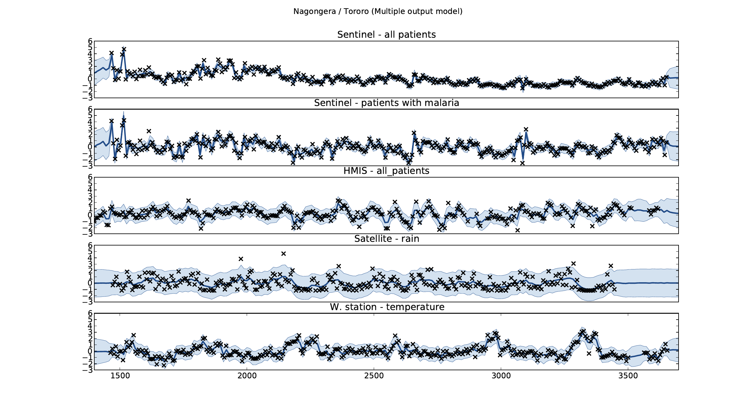
Figure: Sentinel and HMIS data along with rainfall and temperature for the Nagongera sentinel station in the Tororo district.

In collaboration with the AI Research Group at Makerere we chose to investigate whether Gaussian process models could be used to assimilate information from these two different sources of disease informaton. Further, we were interested in whether local information on rainfall and temperature could be used to improve malaria estimates.

The aim of the project was to use WHO Sentinel sites, alongside rainfall and temperature, to improve predictions from HMIS data of levels of malaria.

Figure: The Mubende District.

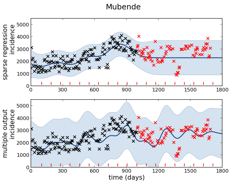
Figure: Prediction of malaria incidence in Mubende.

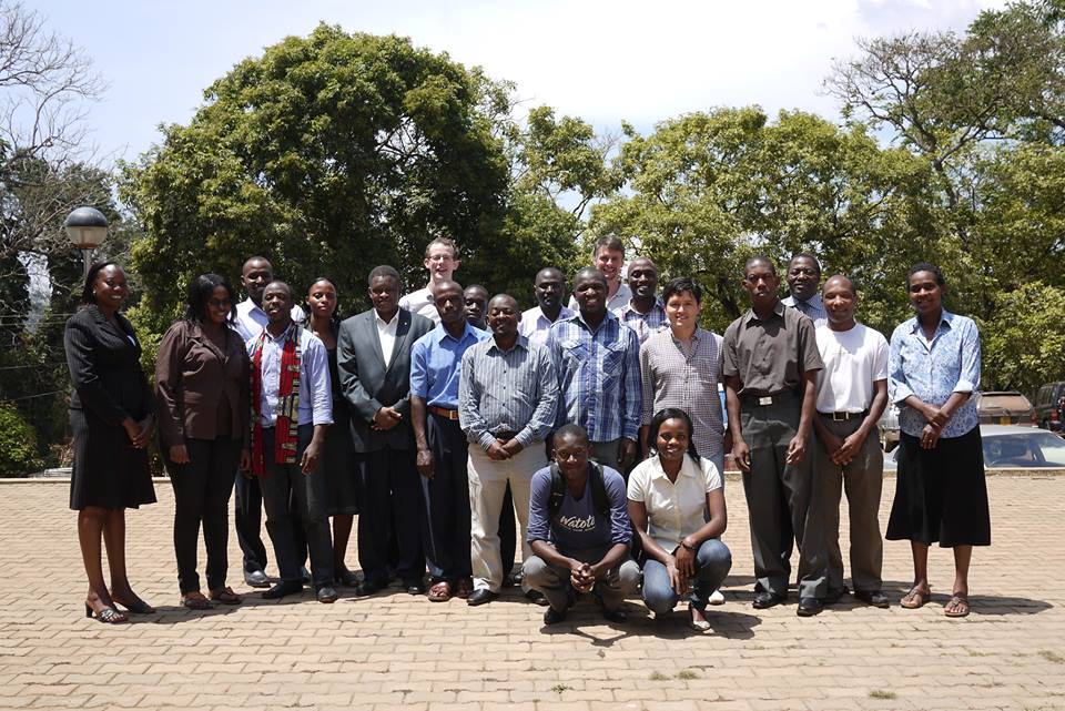
Figure: The project arose out of the Gaussian process summer school held at Makerere in Kampala in 2013. The school led, in turn, to the Data Science Africa initiative.

Early Warning Systems

Figure: The Kabarole district in Uganda.

Figure: Estimate of the current disease situation in the Kabarole district over time. Estimate is constructed with a Gaussian process with an additive covariance funciton.

Health monitoring system for the Kabarole district. Here we have fitted the reports with a Gaussian process with an additive covariance function. It has two components, one is a long time scale component (in red above) the other is a short time scale component (in blue).

Monitoring proceeds by considering two aspects of the curve. Is the blue line (the short term report signal) above the red (which represents the long term trend? If so we have higher than expected reports. If this is the case and the gradient is still positive (i.e. reports are going up) we encode this with a red color. If it is the case and the gradient of the blue line is negative (i.e. reports are going down) we encode this with an amber color. Conversely, if the blue line is below the red and decreasing, we color green. On the other hand if it is below red but increasing, we color yellow.

This gives us an early warning system for disease. Red is a bad situation getting worse, amber is bad, but improving. Green is good and getting better and yellow good but degrading.

Finally, there is a gray region which represents when the scale of the effect is small.

Figure: The map of Ugandan districts with an overview of the Malaria situation in each district.

These colors can now be observed directly on a spatial map of the districts to give an immediate impression of the current status of the disease across the country.

Deep Learning

Classical statistical models and simple machine learning models have a great deal in common. The main difference between the fields is philosophical. Machine learning practitioners are typically more concerned with the quality of prediciton (e.g. measured by ROC curve) while statisticians tend to focus more on the interpretability of the model and the validity of any decisions drawn from that interpretation. For example, a statistical model may be used to validate whether a large scale intervention (such as the mass provision of mosquito nets) has had a long term effect on disease (such as malaria). In this case one of the covariates is likely to be the provision level of nets in a particular region. The response variable would be the rate of malaria disease in the region. The parmaeter, \(\beta_1\) associated with that covariate will demonstrate a positive or negative effect which would be validated in answering the question. The focus in statistics would be less on the accuracy of the response variable and more on the validity of the interpretation of the effect variable, \(\beta_1\).

A machine learning practitioner on the other hand would typically denote the parameter \(w_1\), instead of \(\beta_1\) and would only be interested in the output of the prediction function, \(f(\cdot)\) rather than the parameter itself. The general formalism of the prediction function allows for non-linear models. In machine learning, the emphasis on prediction over interpretability means that non-linear models are often used. The parameters, \(\mathbf{w}\), are a means to an end (good prediction) rather than an end in themselves (interpretable).

DeepFace

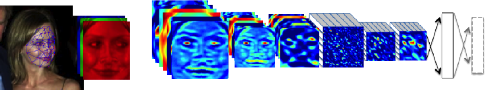
Figure: The DeepFace architecture (Taigman et al., 2014), visualized through colors to represent the functional mappings at each layer. There are 120 million parameters in the model.

The DeepFace architecture (Taigman et al., 2014) consists of layers that deal with translation invariances, known as convolutional layers. These layers are followed by three locally-connected layers and two fully-connected layers. Color illustrates feature maps produced at each layer. The neural network includes more than 120 million parameters, where more than 95% come from the local and fully connected layers.

Deep Learning as Pinball

Figure: Deep learning models are composition of simple functions. We can think of a pinball machine as an analogy. Each layer of pins corresponds to one of the layers of functions in the model. Input data is represented by the location of the ball from left to right when it is dropped in from the top. Output class comes from the position of the ball as it leaves the pins at the bottom.

Sometimes deep learning models are described as being like the brain, or too complex to understand, but one analogy I find useful to help the gist of these models is to think of them as being similar to early pin ball machines.

In a deep neural network, we input a number (or numbers), whereas in pinball, we input a ball.

Think of the location of the ball on the left-right axis as a single number. Our simple pinball machine can only take one number at a time. As the ball falls through the machine, each layer of pins can be thought of as a different layer of ‘neurons’. Each layer acts to move the ball from left to right.

In a pinball machine, when the ball gets to the bottom it might fall into a hole defining a score, in a neural network, that is equivalent to the decision: a classification of the input object.

An image has more than one number associated with it, so it is like playing pinball in a hyper-space.

Figure: At initialization, the pins, which represent the parameters of the function, aren’t in the right place to bring the balls to the correct decisions.

Figure: After learning the pins are now in the right place to bring the balls to the correct decisions.

Learning involves moving all the pins to be in the correct position, so that the ball ends up in the right place when it’s fallen through the machine. But moving all these pins in hyperspace can be difficult.

In a hyper-space you have to put a lot of data through the machine for to explore the positions of all the pins. Even when you feed many millions of data points through the machine, there are likely to be regions in the hyper-space where no ball has passed. When future test data passes through the machine in a new route unusual things can happen.

Adversarial examples exploit this high dimensional space. If you have access to the pinball machine, you can use gradient methods to find a position for the ball in the hyper space where the image looks like one thing, but will be classified as another.

Probabilistic methods explore more of the space by considering a range of possible paths for the ball through the machine. This helps to make them more data efficient and gives some robustness to adversarial examples.

What are Large Language Models?

Probability Conversations

Figure: The focus so far has been on reducing uncertainty to a few representative values and sharing numbers with human beings. We forget that most people can be confused by basic probabilities for example the prosecutor’s fallacy.

In practice we know that probabilities can be very unintuitive, for example in court there is a fallacy known as the “prosecutor’s fallacy” that confuses conditional probabilities. This can cause problems in jury trials (Thompson, 1989).

The MONIAC

The MONIAC was an analogue computer designed to simulate the UK economy. Analogue comptuers work through analogy, the analogy in the MONIAC is that both money and water flow. The MONIAC exploits this through a system of tanks, pipes, valves and floats that represent the flow of money through the UK economy. Water flowed from the treasury tank at the top of the model to other tanks representing government spending, such as health and education. The machine was initially designed for teaching support but was also found to be a useful economic simulator. Several were built and today you can see the original at Leeds Business School, there is also one in the London Science Museum and one in the Unisversity of Cambridge’s economics faculty.

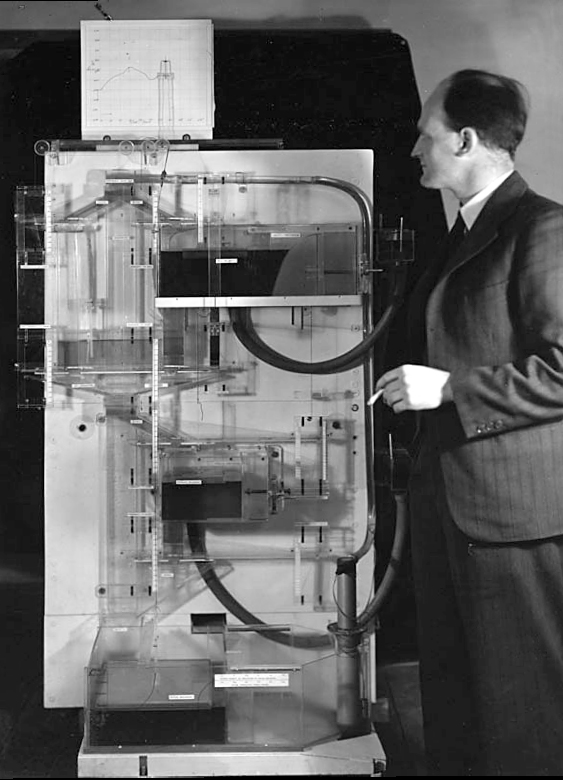
Figure: Bill Phillips and his MONIAC (completed in 1949). The machine is an analogue computer designed to simulate the workings of the UK economy.

Donald MacKay

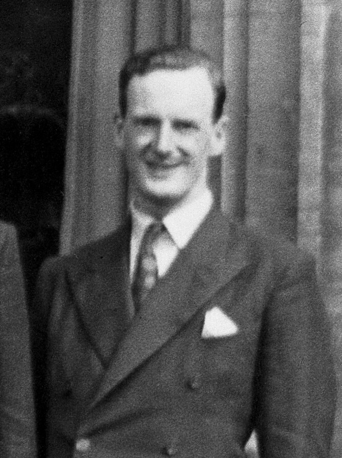
Figure: Donald M. MacKay (1922-1987), a physicist who was an early member of the cybernetics community and member of the Ratio Club.

Donald MacKay was a physicist who worked on naval gun targetting during the second world war. The challenge with gun targetting for ships is that both the target and the gun platform are moving. The challenge was tackled using analogue computers, for example in the US the Mark I fire control computer which was a mechanical computer. MacKay worked on radar systems for gun laying, here the velocity and distance of the target could be assessed through radar and an mechanical electrical analogue computer.

Further Reading

• Section 5.2.2 up to pg 182 of Rogers and Girolami (2011)

Fire Control Systems

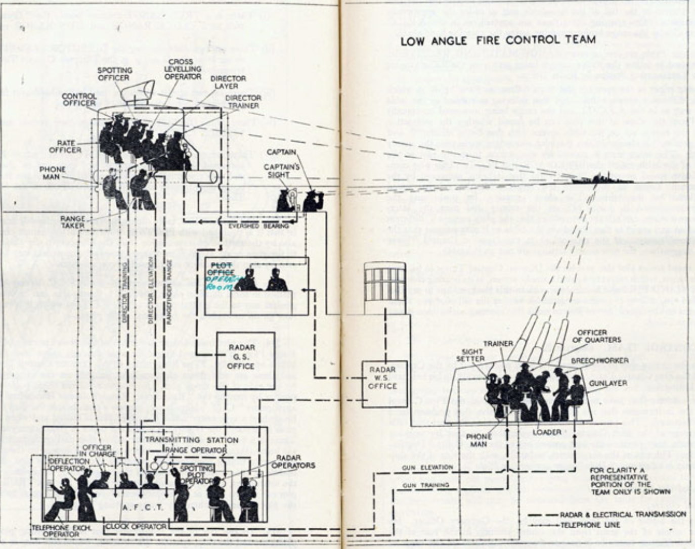
Naval gunnery systems deal with targeting guns while taking into account movement of ships. The Royal Navy’s Gunnery Pocket Book (The Admiralty, 1945) gives details of one system for gun laying.

Like many challenges we face today, in the second world war, fire control was handled by a hybrid system of humans and computers. This means deploying human beings for the tasks that they can manage, and machines for the tasks that are better performed by a machine. This leads to a division of labour between the machine and the human that can still be found in our modern digital ecosystems.

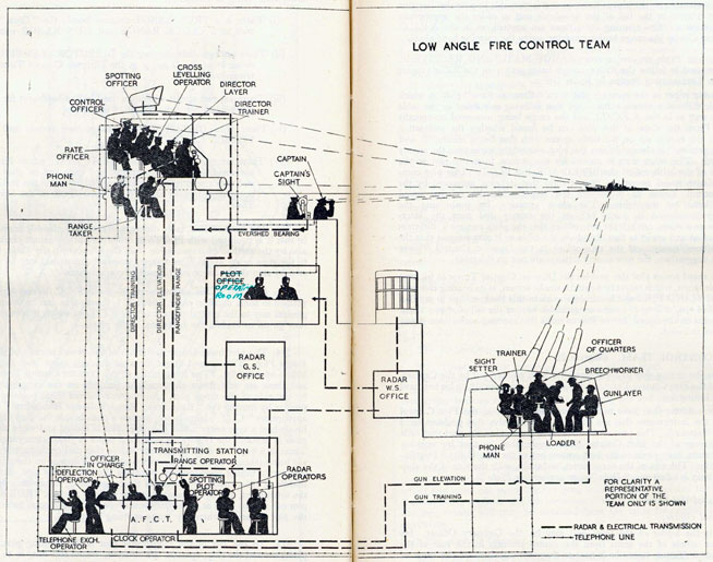
Figure: The fire control computer set at the centre of a system of observation and tracking (The Admiralty, 1945).

As analogue computers, fire control computers from the second world war would contain components that directly represented the different variables that were important in the problem to be solved, such as the inclination between two ships.

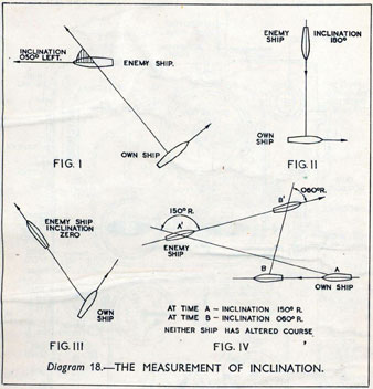
Figure: Measuring inclination between two ships (The Admiralty, 1945). Sophisticated fire control computers allowed the ship to continue to fire while under maneuvers.

The fire control systems were electro-mechanical analogue computers that represented the “state variables” of interest, such as inclination and ship speed with gears and cams within the machine.

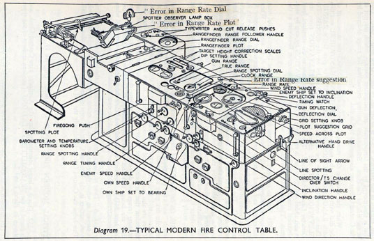
Figure: A second world war gun computer’s control table (The Admiralty, 1945).

For more details on fire control computers, you can watch a 1953 film on the the US the Mark IA fire control computer from Periscope Film.

Figure: U.S. Navy training film MN-6783a. Basic Mechanisms of Fire Control Computers. Mechanical Computer Instructional Film 27794 (1953) for the Mk 1A Fire Control Computer.

Behind the Eye

Figure: Behind the Eye (MacKay, 1991) summarises MacKay’s Gifford Lectures, where MacKay uses the operation of the eye as a window on the operation of the brain.

Donald MacKay was at King’s College for his PhD. He was just down the road from Bill Phillips at LSE who was building the MONIAC. He was part of the Ratio Club. A group of early career scientists who were interested in communication and control in animals and humans, or more specifically they were interested in computers and brains. The were part of an international movement known as cybernetics.

Donald MacKay wrote of the influence that his own work on radar had on his interest in the brain.

… during the war I had worked on the theory of automated and electronic computing and on the theory of information, all of which are highly relevant to such things as automatic pilots and automatic gun direction. I found myself grappling with problems in the design of artificial sense organs for naval gun-directors and with the principles on which electronic circuits could be used to simulate situations in the external world so as to provide goal-directed guidance for ships, aircraft, missiles and the like.

Later in the 1940’s, when I was doing my Ph.D. work, there was much talk of the brain as a computer and of the early digital computers that were just making the headlines as “electronic brains.” As an analogue computer man I felt strongly convinced that the brain, whatever it was, was not a digital computer. I didn’t think it was an analogue computer either in the conventional sense.

But this naturally rubbed under my skin the question: well, if it is not either of these, what kind of system is it? Is there any way of following through the kind of analysis that is appropriate to their artificial automata so as to understand better the kind of system the human brain is? That was the beginning of my slippery slope into brain research.

Behind the Eye pg 40. Edited version of the 1986 Gifford Lectures given by Donald M. MacKay and edited by Valerie MacKay

Importantly, MacKay distinguishes between the analogue computer and the digital computer. As he mentions, his experience was with analogue machines. An analogue machine is literally an analogue. The radar systems that Wiener and MacKay both worked on were made up of electronic components such as resistors, capacitors, inductors and/or mechanical components such as cams and gears. Together these components could represent a physical system, such as an anti-aircraft gun and a plane. The design of the analogue computer required the engineer to simulate the real world in analogue electronics, using dualities that exist between e.g. mechanical circuits (mass, spring, damper) and electronic circuits (inductor, resistor, capacitor). The analogy between mass and a damper, between spring and a resistor and between capacitor and a damper works because the underlying mathematics is approximated with the same linear system: a second order differential equation. This mathematical analogy allowed the designer to map from the real world, through mathematics, to a virtual world where the components reflected the real world through analogy.

Human Analogue Machine

The machine learning systems we have built today that can reconstruct human text, or human classification of images, necessarily must have some aspects to them that are analagous to our understanding. As MacKay suggests the brain is neither a digital or an analogue computer, and the same can be said of the modern neural network systems that are being tagged as “artificial intelligence”.

I believe a better term for them is “human-analogue machines”, because what we have built is not a system that can make intelligent decisions from first principles (a rational approach) but one that observes how humans have made decisions through our data and reconstructs that process. Machine learning is more empiricist than rational, but now we n empirical approach that distils our evolved intelligence.

Figure: The human analogue machine creates a feature space which is analagous to that we use to reason, one way of doing this is to have a machine attempt to compress all human generated text in an auto-regressive manner.

The perils of developing this capability include counterfeit people, a notion that the philosopher Daniel Dennett has described in The Atlantic. This is where computers can represent themselves as human and fool people into doing things on that basis.

LLM Conversations

Figure: The focus so far has been on reducing uncertainty to a few representative values and sharing numbers with human beings. We forget that most people can be confused by basic probabilities for example the prosecutor’s fallacy.

Figure: The Inner Monologue paper suggests using LLMs for robotic planning (Huang et al., 2023).

By interacting directly with machines that have an understanding of human cultural context, it should be possible to share the nature of uncertainty in the same way humans do. See for example the paper Inner Monologue: Embodied Reasoning through Planning Huang et al. (2023).

Intellectual Debt

Figure: Jonathan Zittrain’s term to describe the challenges of explanation that come with AI is Intellectual Debt.

In the context of machine learning and complex systems, Jonathan Zittrain has coined the term “Intellectual Debt” to describe the challenge of understanding what you’ve created. In the ML@CL group we’ve been foucssing on developing the notion of a data-oriented architecture to deal with intellectual debt (Cabrera et al., 2023).

Zittrain points out the challenge around the lack of interpretability of individual ML models as the origin of intellectual debt. In machine learning I refer to work in this area as fairness, interpretability and transparency or FIT models. To an extent I agree with Zittrain, but if we understand the context and purpose of the decision making, I believe this is readily put right by the correct monitoring and retraining regime around the model. A concept I refer to as “progression testing”. Indeed, the best teams do this at the moment, and their failure to do it feels more of a matter of technical debt rather than intellectual, because arguably it is a maintenance task rather than an explanation task. After all, we have good statistical tools for interpreting individual models and decisions when we have the context. We can linearise around the operating point, we can perform counterfactual tests on the model. We can build empirical validation sets that explore fairness or accuracy of the model.

But if we can avoid the pitfalls of counterfeit people, this also offers us an opportunity to psychologically represent (Heider, 1958) the machine in a manner where humans can communicate without special training. This in turn offers the opportunity to overcome the challenge of intellectual debt.

Despite the lack of interpretability of machine learning models, they allow us access to what the machine is doing in a way that bypasses many of the traditional techniques developed in statistics. But understanding this new route for access is a major new challenge.

Figure: The trinity of human, data, and computer, and highlights the modern phenomenon. The communication channel between computer and data now has an extremely high bandwidth. The channel between human and computer and the channel between data and human is narrow. New direction of information flow, information is reaching us mediated by the computer. The focus on classical statistics reflected the importance of the direct communication between human and data. The modern challenges of data science emerge when that relationship is being mediated by the machine.

Figure: The HAM now sits between us and the traditional digital computer.

Networked Interactions

Our modern society intertwines the machine with human interactions. The key question is who has control over these interfaces between humans and machines.

Figure: Humans and computers interacting should be a major focus of our research and engineering efforts.

So the real challenge that we face for society is understanding which systemic interventions will encourage the right interactions between the humans and the machine at all of these interfaces.

Conclusions

In today’s lecture we’ve drilled down further on a difficult aspect of data science. By focusing too much on the data and the technical challenges we face, we can forget the context. But to do data science well, we must not forget the context of the data. We need to pay attention to domain experts and introduce their understanding to our analysis. Above all we must not forget that data is almost always (in the end) about people.

References

Thanks!

For more information on these subjects and more you might want to check the following resources.

• twitter: @lawrennd
• podcast: The Talking Machines
• newspaper: Guardian Profile Page
• blog: http://inverseprobability.com