Week 1: Introduction: ML and the Physical World

[jupyter][google colab][pdf slides]

Neil D. Lawrence

Abstract:

This lecture will introduce the course and provide a motivation and a historical account of machine learning and mathematical modelling. It will further detail the special challenges associated with the application of machine learning to physical systems. We will also outline the objectives of the course and how it will be structured over the term.

Course Overview

Machine Learning and the Physical World is an eight-week course that introduces you to the concepts that are important as we try to use machine learning techniques to better understand the world around us.

Welcome to this course!

• Week 1:
  1. Introduction. Lecturer: Neil D. Lawrence
  2. Quantification of Beliefs. Lecturer: Carl Henrik Ek
• Week 2:
  1. Gaussian processes. Lecturer: Carl Henrik Ek
  2. Simulation. Lecturer: Neil D. Lawrence
• Week 3:
  1. Emulation. Lecturer: Neil D. Lawrence
  2. Sequential Decision Making Under Uncertainty: Bayesian Inference. Lecturer: Carl Henrik Ek
• Week 4:
  1. Probabilistic Numerics. Lecturer: Carl Henrik Ek
  2. Emukit and Experimental Design. Lecturer: Neil D. Lawrence
• Week 5:
  1. Sensitivity Analysis. Lecturer: Neil D. Lawrence
  2. Multifidelity Modelling. Lecturer: Neil D. Lawrence

Special Topics

For weeks 6-8 we will have a series of guest lectures, followed by discussions that will relate the material you have learnt to applications in the real world.

{* Weeks 6-8 will involve three special topics. * In 2023 we had: *

These guest lectures focus on various approaches to simulating the physical world around us, and we will invite you (as part of your mini projects) to consider how important questions around these approaches can be answered as part with the techniques you’ve learnt in the module.

Assessment

There are two forms of assessment. Firstly, we will ask you to a “lab sheet” of answer (based on the notes we provide). The lab can be completed using python and the jupyter notebook (for example on colab). This will be completed by Week 5 and is worth 15%.

We will use the examples we present this year to help inspire a set of mini projects for you to work on in small groups. The aim will be to produce a report on the different challenges, detailing what questions you asked and how you answered them using the techniques we’ll teach. This is submitted first day of Lent term and is worth 85%.

Course Material

Since the breakthrough results in machine learning as applied to tasks in computer vision, speech recognition, language translation, etc., there has been an increasing interest in machine learning techniques as an approach to artificial intelligence.

However, one area where machine learning has (perhaps) made less progress is in those problems where we have a physical understanding of the system.

notutils

This small package is a helper package for various notebook utilities used below.

The software can be installed using

%pip install notutils

from the command prompt where you can access your python installation.

The code is also available on GitHub: https://github.com/lawrennd/notutils

Once notutils is installed, it can be imported in the usual manner.

import notutils

mlai

The mlai software is a suite of helper functions for teaching and demonstrating machine learning algorithms. It was first used in the Machine Learning and Adaptive Intelligence course in Sheffield in 2013.

The software can be installed using

%pip install mlai

from the command prompt where you can access your python installation.

The code is also available on GitHub: https://github.com/lawrennd/mlai

Once mlai is installed, it can be imported in the usual manner.

import mlai

Discovery of Ceres

On New Year’s Eve in 1800, Giuseppe Piazzi, an Italian Priest, born in Lombardy, but installed in a new Observatory at the University viewed a faint smudge through his telescope.

Piazzi was building a star catalogue.

Unbeknownst to him, Piazzi was also participating in an international search. One that he’d been volunteered for by the Hungarian astronomer Franz von Zach. But without even knowing that he’d joined the search party, Piazzi had discovered their target a new planet.

Figure: A blurry image of Ceres taken from the Hubble space telescope. Piazzi first observed the planet while constructing a star catalogue. He was confirming the position of the stars in a second night of observation when he noted one of them was moving. The name planet is originally from the Greek for ‘wanderer’.

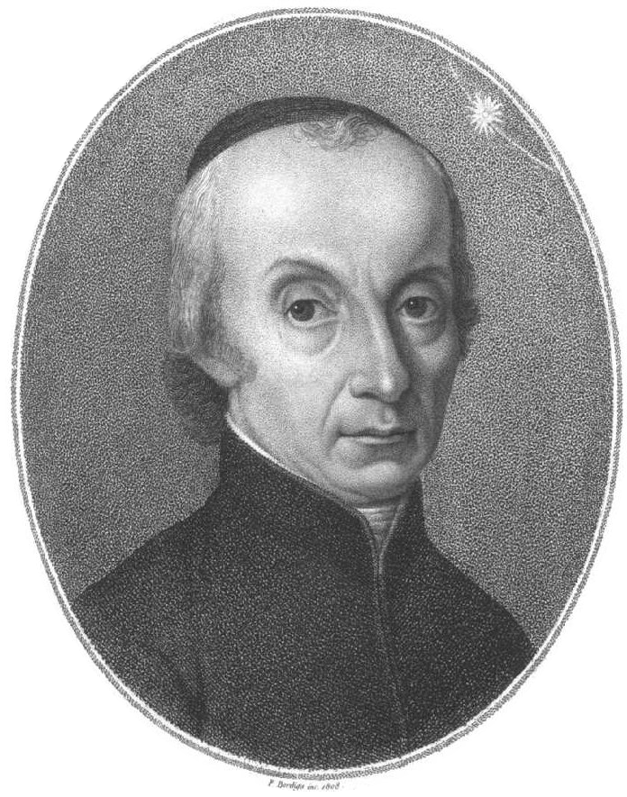
Figure: Giuseppe Piazzi (1746-1826) was an Italian Catholic priest and an astronomer. Jesuits had been closely involved in education, following their surpression in the Kingdom of Naples and Sicily, Piazzi was recruited as part of a drive to revitalize the University of Palermo. His funding was from King Ferdinand I and enabled him to buy high quality instruments from London.

Figure: Announcement of Giuseppe Piazzi’s discovery in the “Monthly Magazine” (also known as the British Register). This announcement is made in August 1801, 7 months after Giuseppe Piazzi first observed Ceres.

The planet’s location was a prediction. It was a missing planet, other planets had been found through a formula, a law, that represented their distance from the sun: \[ a = 0.4 + 0.3 \times 2^m \] where \(m=-\infty, 0, 1, 2, \dots\).

import numpy as np

m = np.asarray([-np.inf, 0, 1, 2, 3, 4, 5, 6])
index = np.asarray(range(len(m)))
planets = ['Mercury', 'Venus', 'Earth', 'Mars', '*', 'Jupiter', 'Saturn', 'Uranus']
a = 0.5 + 0.3*2**m

Figure: The Titius-Bode law was a relatively obscure empirical observation about how the planets are distributed across the solar system. It became well known after the discovery of Uranus by Herschel in 1781 which was found at the location the law predicts for the 8th planet.

When this law was published it fitted all known planets: Mercury, Venus, Earth, Mars, Jupiter and Saturn. Although there was a gap between the fourth and fifth planets (between Mars and Jupiter). In 1781 William Herschel discovered Uranus. It was in the position predicted by the formula. One of the originators of the formula, Johann Elert Bode urged astronomers to search for the missing planet, to be situated between Mars and Jupiter. Franz Xaver von Zach formed the United Astronomical Society, also known as the Celestial Police. But before the celestial police managed to start their search, Piazzi, without even knowing he was a member completed the search. Piazzi first observed the new planet in the early hours of January 1st 1801. He continued to observe it over the next 42 days. Initially he thought it may be a comet, but as he watched it he became convinced he’d found a planet. The international search was over before it started.

Unfortunately, there was a problem. Once he’d found the planet, Piazzi promptly lost it. Piazzi was keen not just to discover the planet, but to to be known as the determiner of its orbit. He took observations across the months of January and February, working to find the orbit. Unfortunately, he was unable to pin it down. He became ill, and by the time the dat awas revealed to the wider community through von Zach’s journal, Monatlicher Correspondenz, the new planet had been lost behind the sun.

Figure: Page from the publication Monatliche Correspondenz that shows Piazzi’s observations of the new planet Piazzi (n.d.) .

%pip install pods

import urllib.request

urllib.request.urlretrieve('http://server3.sky-map.org/imgcut?survey=DSS2&img_id=all&angle=4&ra=3.5&de=17.25&width=1600&height=1600&projection=tan&interpolation=bicubic&jpeg_quality=0.8&output_type=png','ceres-sky-background.png')

import pods

data = pods.datasets.ceres()
right_ascension = data['data']['Gerade Aufstig in Zeit']
declination = data['data']['Nordlich Abweich']

Figure: Plot of the declination and right ascension that Piazzi recorded as Ceres passed through the sky in 1800. Gaps are evenings where Piazzi was unable to make an observation.

Piazzi was able to attempt to predict the orbit because of Kepler’s laws of planetary motion. Johannes Kepler had outlined the way in which planets move according to elliptical shapes, and comets move according to parabolic shapes.

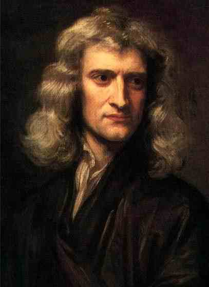
Figure: Godfrey Kneller portrait of Isaac Newton

Later Isaac Newton was able to describe the underlying laws of motion that underpinned Kepler’s laws. This was the enlightenment. An age of science and reason driven by reductionist approaches to the natural world. The enlightenment scientists were able to read and understand each other’s work through the invention of the printing press. Kepler died in 1630, 12 years before Newton was born in 1642. But Kepler’s ideas were able to influence Newton and his peers, and the understanding of gravity became an objective of the nascent Royal Society.

The sharing of information in printed form had evolved by the time of Piazzi, and the collected discoveries of the astronomic world were being shared in Franz von Zach’s monthly journal. It was here that Piazzi’s observations were eventually published, some 7 months after the planet was lost.

It was also here that a young German mathematician read about the international hunt for the lost planet. Carl Friedrich Gauss was a 23-year-old mathematician working from Göttingen. He combined Kepler’s laws with Piazzi’s data to make predictions about where the planet would be found. In doing so, he also developed the method of least squares, and incredibly was able to fit the relatively complex model to the data with a high enough degree of accuracy that astronomers were able to look to the skies to try to recover the planet.

Almost exactly one year after it was lost, Ceres was recovered by Franz von Zach. Gauss had combined model with data to make a prediction and in doing so a new planet was discovered Gauss (1802).

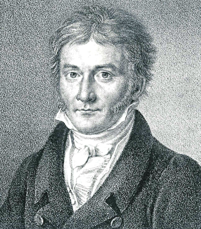
Figure: Carl Friedrich Gauss in 1828. He became internationally famous 27 years earlier for recovering the planet Ceres with a mathematical prediction.

It is this combination of model and data that underpins machine learning but notice that here it has also been delivered through a mechanistic understanding of the way the planets move. This understanding is derived from natural laws that are explicitly incorporated into the model. Kepler’s laws derive from Newton’s mathematical representation of gravity.

But there was a problem. The laws don’t precisely fit the data.

Figure: Gauss’s prediction of Ceres’s orbit as published in Franz von Zach’s Monatliche Correspondenz. He gives the location where the planet may be found, and then some mathematics for making other predictions. He doesn’t share his method, and this later leads to a priority dispute with Legendre around least-squares, which Gauss used to form the fit

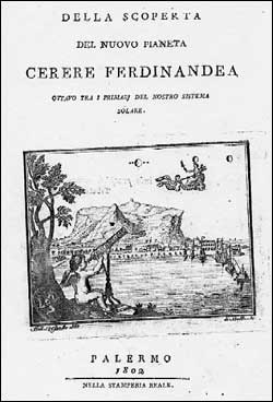
Figure: Piazzi achieved his glory after the planet was discovered. Ceres is an agricultural god (in Greek tradition Demeter). She was associated with Sicily, where Piazzi was working when he made the discovery.

Unfortunately, the story doesn’t end so well for the Titsius-Bode law. In 1846 Neptune was discovered, not in the place predicted by the law (it should be closer to where Pluto was eventually found). And Ceres was found to be merely the largest object in the asteroid belt. It was recategorized as a Dwarf planet.

Figure: The surface area of Ceres is 2,850,000 square kilometers, it’s a little bigger than Greenland, but quite a lot colder. The moon is about 27% of the width of the Earth. Ceres is 7% of the width of the Earth.

Figure: The location of Ceres as ordered in the solar system. While no longer a planet, Ceres is the unique Dwarf Planet in the inner solar system. This image from http://upload.wikimedia.org/wikipedia/commons/c/c4/Planets2008.jpg

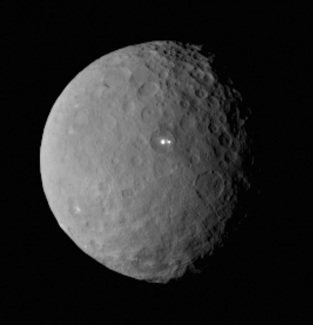
Figure: Ceres as photographed by the Dawn Mission. The photo highlights Ceres’s ‘bright spots’ which are thought to be a material with a high level of reflection (perhaps ice or salt). This image from http://www.popsci.com/sites/popsci.com/files/styles/large_1x_/public/dawn-two-bright-spots.jpg?itok=P5oeSRrc

Let’s have a look at how Gauss determined the orbit of Ceres and how (taking ideas from Pierre Simon Laplace) he used approaches that would prove to be conceptually fundamental to machine learning and statistical approaches.

Overdetermined System

The challenge with a linear model is that it has two unknowns, \(m\), and \(c\). Observing data allows us to write down a system of simultaneous linear equations. So, for example if we observe two data points, the first with the input value, \(x_1 = 1\) and the output value, \(y_1 =3\) and a second data point, \(x= 3\), \(y=1\), then we can write two simultaneous linear equations of the form.

point 1: \(x= 1\), \(y=3\) \[ 3 = m + c \] point 2: \(x= 3\), \(y=1\) \[ 1 = 3m + c \]

The solution to these two simultaneous equations can be represented graphically as

Figure: The solution of two linear equations represented as the fit of a straight line through two data

The challenge comes when a third data point is observed, and it doesn’t fit on the straight line.

point 3: \(x= 2\), \(y=2.5\) \[ 2.5 = 2m + c \]

Figure: A third observation of data is inconsistent with the solution dictated by the first two observations

Now there are three candidate lines, each consistent with our data.

Figure: Three solutions to the problem, each consistent with two points of the three observations

This is known as an overdetermined system because there are more data than we need to determine our parameters. The problem arises because the model is a simplification of the real world, and the data we observe is therefore inconsistent with our model.

Pierre-Simon Laplace

The solution was proposed by Pierre-Simon Laplace. His idea was to accept that the model was an incomplete representation of the real world, and the way it was incomplete is unknown. His idea was that such unknowns could be dealt with through probability.

Pierre-Simon Laplace

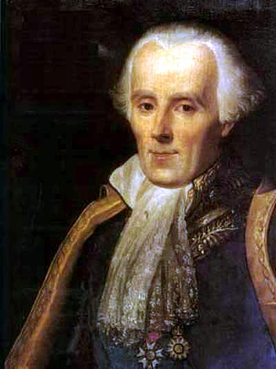
Figure: Pierre-Simon Laplace 1749-1827.

Laplace’s Demon

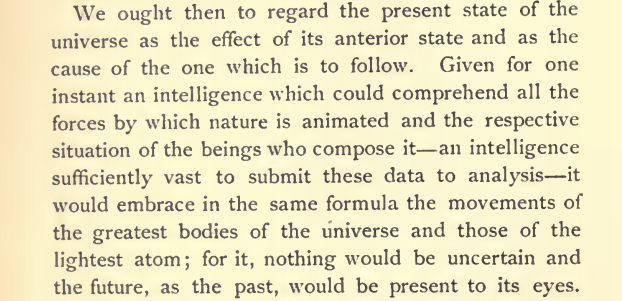
Figure: English translation of Laplace’s demon, taken from the Philosophical Essay on probabilities Laplace (1814) pg 3.

One way of viewing what Laplace is saying is that we can take “the forces by which nature is animated” or our best mathematical/computational abstraction of that which we would call the model and combine it with the “respective situation of the beings who compose it” which I would refer to as the data and if we have an “intelligence sufficiently vast enough to submit these data to analysis”, or sufficient compute then we would have a system for which “nothing would be uncertain and the future, as the past, would be present in its eyes”, or in other words we can make a prediction. Or more succinctly put we have

Laplace’s demon has been a recurring theme in science, we can also find it in Stephen Hawking’s book A Brief History of Time (A brief history of time, 1988).

If we do discover a theory of everything … it would be the ultimate triumph of human reason-for then we would truly know the mind of God

Stephen Hawking in A Brief History of Time 1988

But is it really that simple? Do we just need more and more accurate models and more and more data?

Laplace’s Gremlin

The curve described by a simple molecule of air or vapor is regulated in a manner just as certain as the planetary orbits; the only difference between them is that which comes from our ignorance. Probability is relative, in part to this ignorance, in part to our knowledge. We know that of three or greater number of events a single one ought to occur; but nothing induces us to believe that one of them will occur rather than the others. In this state of indecision it is impossible for us to announce their occurrence with certainty. It is, however, probable that one of these events, chosen at will, will not occur because we see several cases equally possible which exclude its occurrence, while only a single one favors it.

— Pierre-Simon Laplace (Laplace, 1814), pg 5

The representation of ignorance through probability is the true message of Laplace, I refer to this message as “Laplace’s gremlin”, because it is the gremlin of uncertainty that interferes with the demon of determinism to mean that our predictions are not deterministic.

Our separation of the uncertainty into the data, the model and the computation give us three domains in which our doubts can creep into our ability to predict. Over the last three lectures we’ve introduced some of the basic tools we can use to unpick this uncertainty. You’ve been introduced to, (or have yow reviewed) Bayes’ rule. The rule, which is a simple consequence of the product rule of probability, is the foundation of how we update our beliefs in the presence of new information.

The real point of Laplace’s essay was that we don’t have access to all the data, we don’t have access to a complete physical understanding, and as the example of the Game of Life shows, even if we did have access to both (as we do for “Conway’s universe”) we still don’t have access to all the compute that we need to make deterministic predictions. There is uncertainty in the system which means we can’t make precise predictions.

Gremlins are imaginary creatures used as an explanation of failure in aircraft, causing crashes. In that sense the Gremlin represents the uncertainty that a pilot felt about what might go wrong in a plane which might be “theoretically sound” but in practice is poorly maintained or exposed to conditions that take it beyond its design criteria. Laplace’s gremlin is all the things that your model, data and ability to compute don’t account for bringing about failures in your ability to predict. Laplace’s gremlin is the uncertainty in the system.

Figure: Gremlins are seen as the cause of a number of challenges in this World War II poster.

Laplace’s concept was that the reason that the data doesn’t match up to the model is because of unconsidered factors, and that these might be well represented through probability densities. He tackles the challenge of the unknown factors by adding a variable, \(\epsilon\), that represents the unknown. In modern parlance we would call this a latent variable. But in the context Laplace uses it, the variable is so common that it has other names such as a “slack” variable or the noise in the system.

point 1: \(x= 1\), \(y=3\) \[ 3 = m + c + \epsilon_1 \] point 2: \(x= 3\), \(y=1\) \[ 1 = 3m + c + \epsilon_2 \] point 3: \(x= 2\), \(y=2.5\) \[ 2.5 = 2m + c + \epsilon_3 \]

Laplace’s trick has converted the overdetermined system into an underdetermined system. He has now added three variables, \(\{\epsilon_i\}_{i=1}^3\), which represent the unknown corruptions of the real world. Laplace’s idea is that we should represent that unknown corruption with a probability distribution.

A Probabilistic Process

However, it was left to an admirer of Laplace to develop a practical probability density for that purpose. It was Carl Friedrich Gauss who suggested that the Gaussian density (which at the time was unnamed!) should be used to represent this error.

The result is a noisy function, a function which has a deterministic part, and a stochastic part. This type of function is sometimes known as a probabilistic or stochastic process, to distinguish it from a deterministic process.

Hydrodynamica

When Laplace spoke of the curve of a simple molecule of air, he may well have been thinking of Daniel Bernoulli (1700-1782). Daniel Bernoulli was one name in a prodigious family. His father and brother were both mathematicians. Daniel’s main work was known as Hydrodynamica.

Figure: Daniel Bernoulli’s Hydrodynamica published in 1738. It was one of the first works to use the idea of conservation of energy. It used Newton’s laws to predict the behaviour of gases.

Daniel Bernoulli described a kinetic theory of gases, but it wasn’t until 170 years later when these ideas were verified after Einstein had proposed a model of Brownian motion which was experimentally verified by Jean Baptiste Perrin.

Figure: Daniel Bernoulli’s chapter on the kinetic theory of gases, for a review on the context of this chapter see Mikhailov (n.d.). For 1738 this is extraordinary thinking. The notion of kinetic theory of gases wouldn’t become fully accepted in Physics until 1908 when a model of Einstein’s was verified by Jean Baptiste Perrin.

Entropy Billiards

Entropy:

New Ball Pause Skip 1000s Histogram

Figure: Bernoulli’s simple kinetic models of gases assume that the molecules of air operate like billiard balls.

import numpy as np

p = np.random.randn(10000, 1)
xlim = [-4, 4]
x = np.linspace(xlim[0], xlim[1], 200)
y = 1/np.sqrt(2*np.pi)*np.exp(-0.5*x*x)

Another important figure for Cambridge was the first to derive the probability distribution that results from small balls banging together in this manner. In doing so, James Clerk Maxwell founded the field of statistical physics.

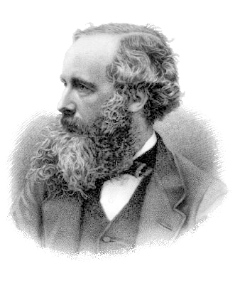
Figure: James Clerk Maxwell 1831-1879 Derived distribution of velocities of particles in an ideal gas (elastic fluid).

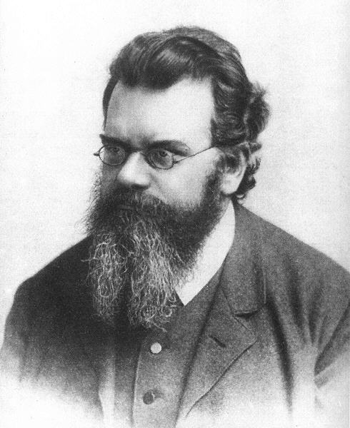
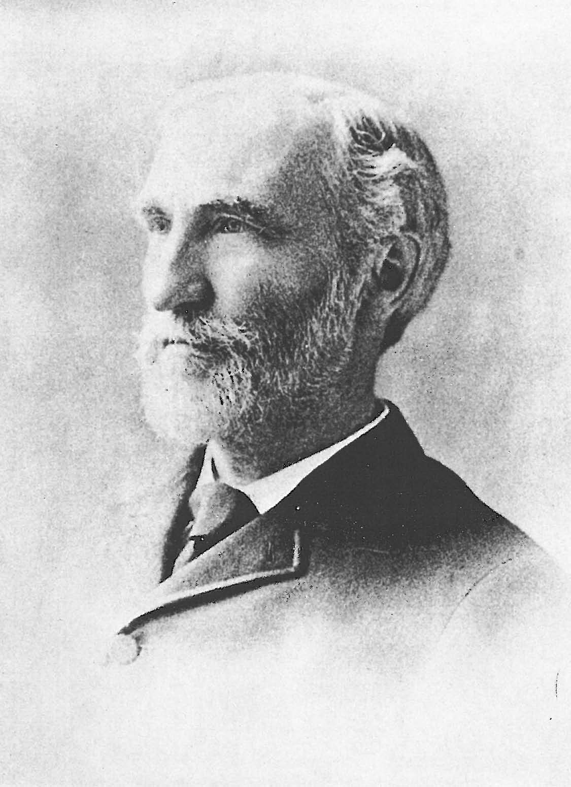
Figure: James Clerk Maxwell (1831-1879), Ludwig Boltzmann (1844-1906) Josiah Willard Gibbs (1839-1903)

Many of the ideas of early statistical physicists were rejected by a cadre of physicists who didn’t believe in the notion of a molecule. The stress of trying to have his ideas established caused Boltzmann to commit suicide in 1906, only two years before the same ideas became widely accepted.

Figure: Boltzmann’s paper Boltzmann (n.d.) which introduced the relationship between entropy and probability. A translation with notes is available in Sharp and Matschinsky (2015).

The important point about the uncertainty being represented here is that it is not genuine stochasticity, it is a lack of knowledge about the system. The techniques proposed by Maxwell, Boltzmann and Gibbs allow us to exactly represent the state of the system through a set of parameters that represent the sufficient statistics of the physical system. We know these values as the volume, temperature, and pressure. The challenge for us, when approximating the physical world with the techniques we will use is that we will have to sit somewhere between the deterministic and purely stochastic worlds that these different scientists described.

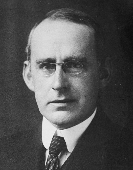
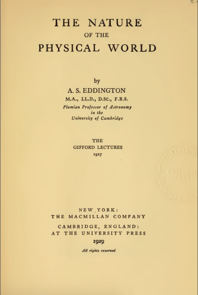
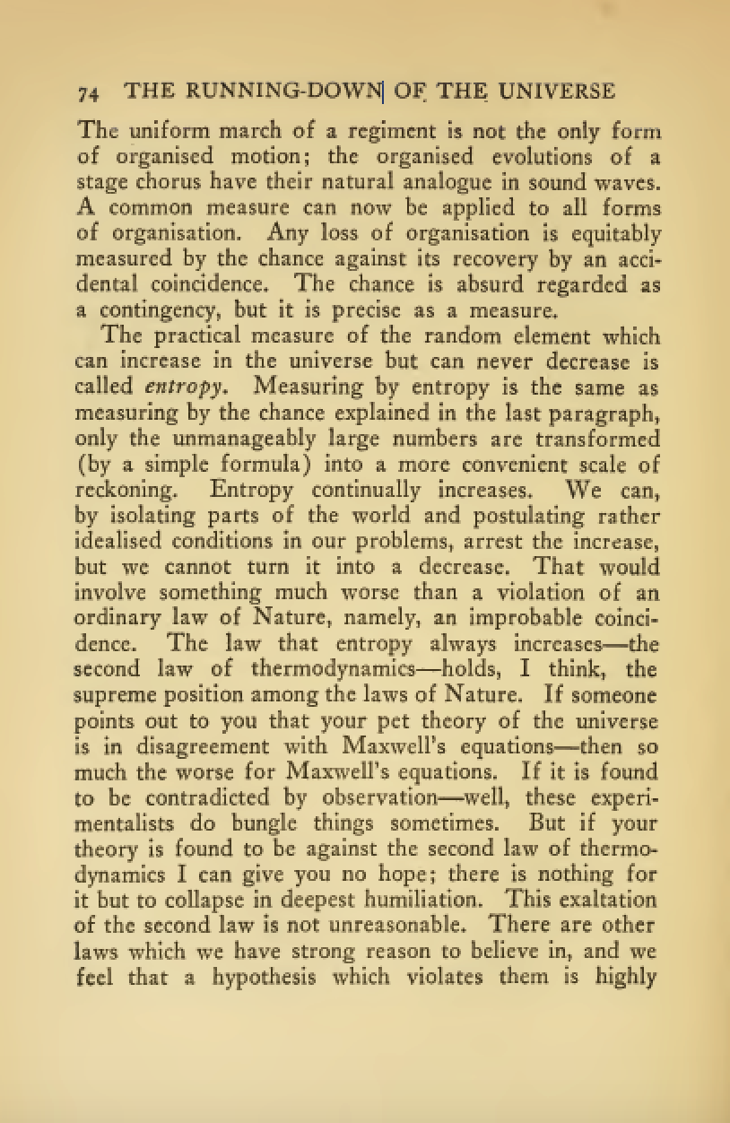
One ongoing characteristic of people who study probability and uncertainty is the confidence with which they hold opinions about it. Another leader of the Cavendish laboratory expressed his support of the second law of thermodynamics (which can be proven through the work of Gibbs/Boltzmann) with an emphatic statement at the beginning of his book.

Figure: Eddington’s book on the Nature of the Physical World (Eddington, 1929)

The same Eddington is also famous for dismissing the ideas of a young Chandrasekhar who had come to Cambridge to study in the Cavendish lab. Chandrasekhar demonstrated the limit at which a star would collapse under its own weight to a singularity, but when he presented the work to Eddington, he was dismissive suggesting that there “must be some natural law that prevents this abomination from happening”.

Figure: Chandrasekhar (1910-1995) derived the limit at which a star collapses in on itself. Eddington’s confidence in the 2nd law may have been what drove him to dismiss Chandrasekhar’s ideas, humiliating a young scientist who would later receive a Nobel prize for the work.

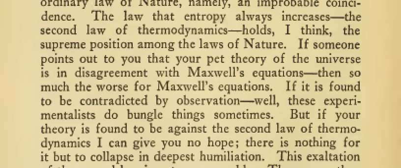
Figure: Eddington makes his feelings about the primacy of the second law clear. This primacy is perhaps because the second law can be demonstrated mathematically, building on the work of Maxwell, Gibbs and Boltzmann. Eddington (1929)

Presumably he meant that the creation of a black hole seemed to transgress the second law of thermodynamics, although later Hawking was able to show that blackholes do evaporate, but the time scales at which this evaporation occurs is many orders of magnitude slower than other processes in the universe.

Underdetermined System

What about the situation where you have more parameters than data in your simultaneous equation? This is known as an underdetermined system. In fact, this set up is in some sense easier to solve, because we don’t need to think about introducing a slack variable (although it might make a lot of sense from a modelling perspective to do so).

The way Laplace proposed resolving an overdetermined system, was to introduce slack variables, \(\epsilon_i\), which needed to be estimated for each point. The slack variable represented the difference between our actual prediction and the true observation. This is known as the residual. By introducing the slack variable, we now have an additional \(n\) variables to estimate, one for each data point, \(\{\epsilon_i\}\). This turns the overdetermined system into an underdetermined system. Introduction of \(n\) variables, plus the original \(m\) and \(c\) gives us \(n+2\) parameters to be estimated from \(n\) observations, which makes the system underdetermined. However, we then made a probabilistic assumption about the slack variables, we assumed that the slack variables were distributed according to a probability density. And for the moment we have been assuming that density was the Gaussian, \[\epsilon_i \sim \mathcal{N}\left(0,\sigma^2\right),\] with zero mean and variance \(\sigma^2\).

The follow up question is whether we can do the same thing with the parameters. If we have two parameters and only one unknown, can we place a probability distribution over the parameters as we did with the slack variables? The answer is yes.

Underdetermined System

Figure: An underdetermined system can be fit by considering uncertainty. Multiple solutions are consistent with one specified point.

Brownian Motion and Wiener

Robert Brown was a botanist who was studying plant pollen in 1827 when he noticed a trembling motion of very small particles contained within cavities within the pollen. He worked hard to eliminate the potential source of the movement by exploring other materials where he found it to be continuously present. Thus, the movement was not associated, as he originally thought, with life.

In 1905 Albert Einstein produced the first mathematical explanation of the phenomenon. This can be seen as our first model of a ‘curve of a simple molecule of air’. To model the phenomenon Einstein introduced stochasticity to a differential equation. The particles were being peppered with high-speed water molecules, that was triggering the motion. Einstein modelled this as a stochastic process.

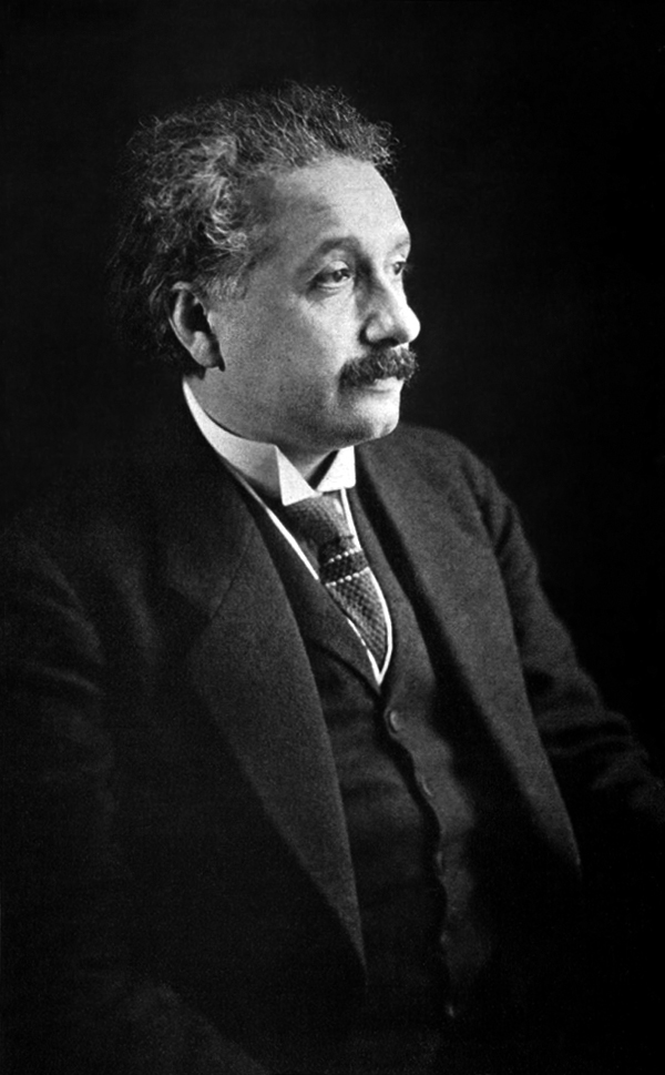
Figure: Albert Einstein’s 1905 paper on Brownian motion introduced stochastic differential equations which can be used to model the ‘curve of a simple molecule of air’.

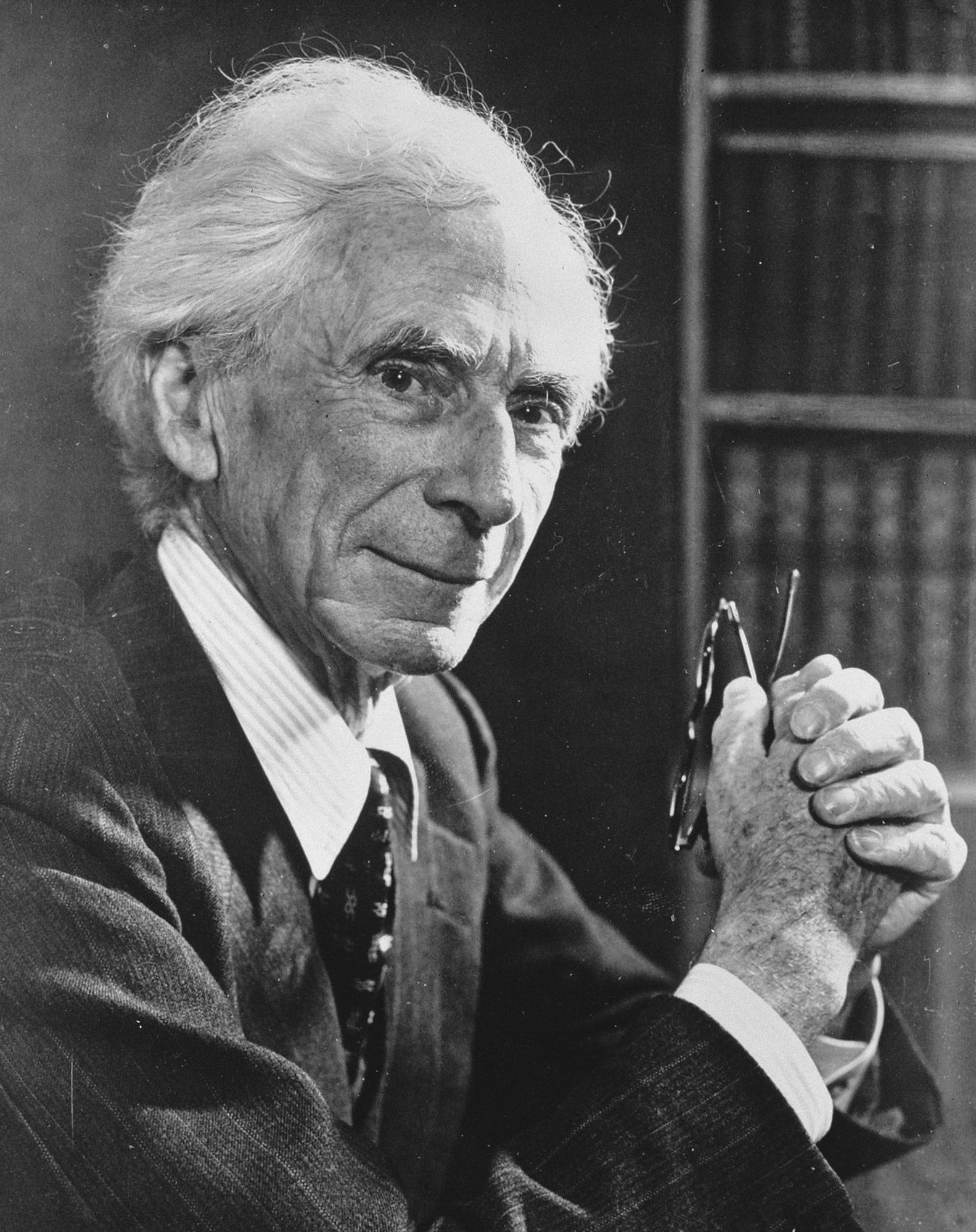
Norbert Wiener was a child prodigy, whose father had schooled him in philosophy. He was keen to have his son work with the leading philosophers of the age, so at the age of 18 Wiener arrived in Cambridge (already with a PhD). He was despatched to study with Bertrand Russell but Wiener and Russell didn’t get along. Wiener wasn’t persuaded by Russell’s ideas for theories of knowledge through logic. He was more aligned with Laplace and his desire for a theory of ignorance. In is autobiography he relates it as the first thing he could see his father was proud of (at around the age of 10 or 11) (Wiener, 1953).

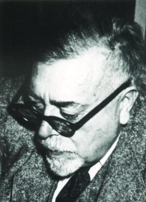
Figure: Bertrand Russell (1872-1970), Albert Einstein (1879-1955), Norbert Wiener, (1894-1964)

But Russell (despite also not getting along well with Wiener) introduced Wiener to Einstein’s works, and Wiener also met G. H. Hardy. He left Cambridge for Göttingen where he studied with Hilbert. He developed the underlying mathematics for proving the existence of the solutions to Einstein’s equation, which are now known as Wiener processes.

Figure: Brownian motion of a large particle in a group of smaller particles. The movement is known as a Wiener process after Norbert Wiener.

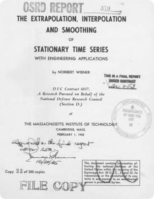
Figure: Norbert Wiener (1894 - 1964). Founder of cybernetics and the information era. He used Gibbs’s ideas to develop a “theory of ignorance” that he deployed in early communication. On the right is Wiener’s wartime report that used stochastic processes in forecasting with applications in radar control (image from Coales and Kane (2014)).

Wiener himself used the processes in his work. He was focused on mathematical theories of communication. Between the world wars he was based at Massachusetts Institute of Technology where the burgeoning theory of electrical engineering was emerging, with a particular focus on communication lines. Winer developed theories of communication that used Gibbs’s entropy to encode information. He also used the ideas behind the Wiener process for developing tracking methods for radar systems in the second world war. These processes are what we know of now as Gaussian processes (Wiener (1949)).

Conclusions

In this introduction to the course, we’ve provided a potted journey through the history of science and our models of the physical world. We started with the deterministic world of Newton and moved towards a less certain, stochastic world, beautifully described by Laplace.

Within statistical mechanics and electrical engineering, the ideas of Laplace were rendered into mathematical reality. In particular, through the use of probabilistic processes such as Gaussian processes.

The challenge we face is one of partial ignorance. Not the total ignorance of Maxwell/Gibbs/Boltzmann or the determinism of Newton. But something in between.

In this course, that ignorance won’t only arise from lack of observation, but also from the need to run a (potentially) expensive simulation. Our aim will be to introduce you to the ideas of surrogate modeling, that allow us to trade off our current knowledge, with our possible knowledge, where data can be acquired through observation or simulation to render an answer to a question.

In the next set of lectures, you will obtain a more rigorous grounding in uncertainty and the mathematics and creation of Gaussian process models. We will then use these tools to show how a range of decisions can be made through combination of these surrogate models with simulations.

Thanks!

For more information on these subjects and more you might want to check the following resources.

• book: The Atomic Human
• twitter: @lawrennd
• podcast: The Talking Machines
• newspaper: Guardian Profile Page
• blog: http://inverseprobability.com

References