Practical 5: Clustering Chimpanzees

Abstract

In this self-guided practical we showcase a practical example of K-means clustering on Chimpanzee faces. Using a pre-trained classifier to generate a vector encoding of each portrait, we analyse the best parameter selection, and finally, implement K-means clustering.

Chimpanzee Faces

We know that human faces are unique to each of us. But did you know that chimpanzees also have unique faces?

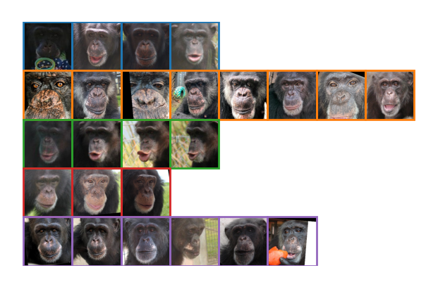
We will be checking if different images of the same chimpanzee would naturally cluster together. Using a sample set of 25 photos of 5 chimpanzees from Iashin et al., 2025, let’s see if we are able to cluster the dataset.

Let’s download the photos (and other code we will need later). The ChimpUFE repo was created by Iashin et al. We will also be using their pre-trained neural networks for creating embeddings of the chimp’s faces.

Iashin, Vladimir, et al. “Self-supervised Learning on Camera Trap Footage Yields a Strong Universal Face Embedder.” arXiv preprint arXiv:2507.10552 (2025).

#these files are quite large and take a couple minutes to download
!git clone https://github.com/v-iashin/ChimpUFE.git
!cd ChimpUFE && pip install -r requirements.txt
!wget -P ./ChimpUFE/assets/weights https://github.com/v-iashin/ChimpUFE/releases/download/v1.0/25-06-06T20-51-36_330k.pth

This is what the chimps look like:

\(k\) Means Clustering

Let’s use the images directly to try to cluster the pictures. After extracting the pixel values, we will apply dimensionality reduction so that we can visualise the process.

import os
import numpy as np
import matplotlib.image as mpimg

paths = [os.path.join(gallery, f, img)
         for f in sorted(os.listdir(gallery))
         for img in sorted(os.listdir(os.path.join(gallery, f)))]

images = np.array([mpimg.imread(p).ravel() for p in paths])
print(images.shape)

from sklearn.decomposition import PCA

images_2d = PCA(n_components=2).fit_transform(images)
print(images_2d.shape)

Let’s visualise our 2d mapping of the chimps. We can see that for the most part it’s not the worst, with many similar photos grouped together, but it’s surely not going to allow us to perfectly separate them.

import matplotlib.pyplot as plt
from matplotlib.offsetbox import OffsetImage, AnnotationBbox
import matplotlib.image as mpimg

fig, ax = plt.subplots(figsize=(6,6))

target_px = 32

for (x, y), path in zip(images_2d, paths):
    img = mpimg.imread(path)
    h, w = img.shape[:2]
    zoom = target_px / max(h, w)
    ab = AnnotationBbox(OffsetImage(img, zoom=zoom), (x, y), frameon=False)
    ax.add_artist(ab)

mins = images_2d.min(axis=0); maxs = images_2d.max(axis=0)
pad = 0.05 * (maxs - mins)
ax.set_xlim(mins[0]-pad[0], maxs[0]+pad[0])
ax.set_ylim(mins[1]-pad[1], maxs[1]+pad[1])
ax.set_xticks([]); ax.set_yticks([])

K-Means

We will now apply K-means clustering on the mappings to group similar faces together.

Let’s implement the algorithm as presented in the lecture.

1.  First, initialize cluster centres by randomly selecting k data points
2.  Assign each data point to its nearest cluster centre
3.  Update each cluster centre by computing the mean of all points assigned to it
4.  Repeat steps 2 and 3 until the cluster assignments stop changing

Exercise 1

Now, let’s implement K-means clustering. Let’s avoid using scikit-learn’s KMeans, or another imported library, as we want to implement it fram scratch, and visualise all the steps.

Use the widget below to visualise the progress of your K-means clustering.

import numpy as np
import matplotlib.pyplot as plt
import ipywidgets as widgets
from IPython.display import display
from sklearn.decomposition import PCA
import matplotlib.image as mpimg

X2, history_i2d = iterative_kmeans_widget(images_2d, paths)

Performance

Reasoning about clustering performance is very diffucult, as there will often not be a simple cluster-class relationship, which will make it hard to say what image should be where. Many metrics exist, but none are perfect.

Two approaches we will use here are: - Force a cluster-class correspondence by finding the permutation with the best accuracy. - Adjusted Rand Index (ARI) - counting pairs of images from the same class in the same cluster, adjusting for random chance.

from sklearn.metrics import adjusted_rand_score
import itertools

classes = [x.split('/')[-2] for x in paths]
performance_stats(history_i2d, classes)

Both measures report that we did do better than random chance, but not by a lot. We can definetely improve on this, as pixel values taken alone do not carry sufficient information. To show this more intuitively - our approach didn’t even take into account which pixels were next to each other!

Face Embeddings

This is where Neural Networks have a significant advantage, and we can use them to improve on the very naive clustering we did above. We will be using a pre-trained model provided by Iashin et al. These embeddings encode high-level facial features in a numerical vector space.

We will now extract the embeddings for these 25 images.

import os
import torch
from PIL import Image
from torch.utils.data import DataLoader
from torchvision import datasets

embeddings = make_embeddings('./assets/gallery')
print(embeddings.shape)

To be able to intuitively reason about the clustering and visualise it, we will again use dimensionality reduction to convert the encodings into 2 dimensions. Note, that this will hurt performance, as we’re discarding most of the information.

embeddings_2d = PCA(n_components=2).fit_transform(embeddings)

And now, we can reuse the code we wrote above to see if the clustering works better on the embeddings. It should!

X2, history_e2d = iterative_kmeans_widget(embeddings_2d, paths, random_state=2)
# the reason i'm fiddling with random state is because quite often the clustering succeeds in 1 step, which is not very illustrative

And we again evaluate performance. The raw pixel value PCA achieved about 0.44 best accuracy and 0.13 ARI. Do we do better?

performance_stats(history_e2d, classes)

Ee lost quite a lot of information by boiling everything down to 2 dimensions. For completeness, let’s repeat the 2 above analyses without the PCA step - bear in mind that this will make the visualisations quite a bit useless, so we’ll skip it.

print('Full Images')
history_i = cluster_kmeans_handwritten(images, 5)
performance_stats(history_i, classes)
print('Full Embeddings')
history_e = cluster_kmeans_handwritten(np.array(embeddings), 5)
performance_stats(history_e, classes)

Looks like there’s no big improvement, and actually, the PCA images beats full images! While the lack of improvement on 2d embeddings is unexpected (and probably with more data we would see a significant differences), the 2d PCA over raw images is actually expected to do better. Why?

Other datasets

Another bigger dataset of labeled chimpanzee images was published here: paper, github.

Alexander Freytag and Erik Rodner and Marcel Simon and Alexander Loos and Hjalmar Kühl and Joachim Denzler: “Chimpanzee Faces in the Wild: Log-Euclidean CNNs for Predicting Identities and Attributes of Primates,” German Conference on Pattern Recognition (GCPR), 2016 .

!git clone https://github.com/cvjena/chimpanzee_faces.git

The below text file contains a description of the dataset. We’re selecting only the Filename and Name, but you might use more data in other analyses. The below code converts it into a handy dataframe.

import pandas as pd

ann = "chimpanzee_faces/datasets_cropped_chimpanzee_faces/data_CTai/annotations_ctai.txt" # you can also use data_CZoo
with open(ann) as f:
  recs = [{line.strip().split()[i]: line.strip().split()[i+1] for i in [0, 2]} for line in f]
df_freytag = pd.DataFrame(recs)
df_freytag

Exercise 2

Assess the data, and modify it as necessary

Let’s select a subset of this, to use in our clusterings.

import random
import shutil

def sample_subset(df, n, min_, max_=None, seed=42):
    if max_ is None:
      max_ = min_
    rng = random.Random(seed)
    valid = [n for n, c in df["Name"].value_counts().items() if c >= min_]
    names = rng.sample(valid, n)
    dfs = []
    for name in names:
        sub = df[df["Name"] == name]
        n = rng.randint(min_, min(max_, len(sub)))
        dfs.append(sub.sample(n, random_state=seed))
    out = pd.concat(dfs)
    return out

df_freytag_small = sample_subset(df_freytag, 10, 10) # 10 photos each for 10 chimps

gallery_freytag = "ChimpUFE/assets/gallery_freytag"
os.makedirs(gallery_freytag, exist_ok=True)
base = "chimpanzee_faces/datasets_cropped_chimpanzee_faces/data_CTai"

for _, row in df_freytag_small.iterrows():
    identity = row["Name"]
    src = os.path.join(base, row["Filename"])
    os.makedirs(os.path.join(gallery_freytag, identity), exist_ok=True)
    dst = os.path.join(gallery_freytag, identity, os.path.basename(row["Filename"]))
    shutil.copy(src, dst)

paths_freytag = [os.path.join(gallery_freytag, f, img)
         for f in sorted(os.listdir(gallery_freytag))
         for img in sorted(os.listdir(os.path.join(gallery_freytag, f)))]

df_freytag_small

Finally, we can run the same embedding code on the new dataset.

embeddings_freytag = make_embeddings('./assets/gallery_freytag')

embeddings_freytag_2d = PCA(n_components=2).fit_transform(embeddings_freytag)

X2, history_freytag_e2d = iterative_kmeans_widget(embeddings_freytag_2d, paths_freytag, n_clusters=10, random_state=42)

classes_freytag = df_freytag_small['Name'].values
performance_stats(history_freytag_e2d, classes_freytag)

The adjusted Rand index tells us that our approach worked on the new dataset!

Hierarchical Clustering

Hierarchical clustering is an alternative method, where all elements are at first considered their own clusters, and repetetively join the closest clusters together, until only one remains. This is very nicely visualised using dendrograms.

Exercise 3

Using our earlier dataset, let’s conduct hierarchical clustering, and produce a dendrogram.

from matplotlib.offsetbox import OffsetImage, AnnotationBbox
from scipy.cluster.hierarchy import dendrogram

linkage_output = cluster_hierarchical_handwritten(embeddings_2d)
show_dendrogram(linkage_output, paths)

End of Practical 5

 _______  __   __  _______  __    _  ___   _  _______  __
|       ||  | |  ||   _   ||  |  | ||   | | ||       ||  |
|_     _||  |_|  ||  |_|  ||   |_| ||   |_| ||  _____||  |
  |   |  |       ||       ||       ||      _|| |_____ |  |
  |   |  |       ||       ||  _    ||     |_ |_____  ||__|
  |   |  |   _   ||   _   || | |   ||    _  | _____| | __
  |___|  |__| |__||__| |__||_|  |__||___| |_||_______||__|

Thanks!

For more information on these subjects and more you might want to check the following resources.

• company: Trent AI
• book: The Atomic Human
• twitter: @lawrennd
• podcast: The Talking Machines
• newspaper: Guardian Profile Page
• blog: http://inverseprobability.com