Week 4: Deep Architectures

[jupyter][google colab][reveal]

Neil Lawrence

Abstract:

This lecture will explore what happens when we compose layers of basis functions together to form deep neural networks..

%pip install daft-pgm

ML Foundations Course Notebook Setup

We install some bespoke codes for creating and saving plots as well as loading data sets.

%%capture
%pip install notutils
%pip install git+https://github.com/lawrennd/ods.git
%pip install git+https://github.com/lawrennd/mlai.git

import notutils
import pods
import mlai
import mlai.plot as plot

Review

By this point in the course we have covered the foundations sufficiently for you to look at three Cambridge courses.

• Advanced Data Science
• ML and the Physical World
• Deep Neural Networks

Today we will give some insight into the third of those courses, deep neural networks.

Basis Functions to Neural Networks

From Basis Functions to Neural Networks

So far, we have been talking about linear models or shallow learning as we might think of it. Let’s pause for a moment and consider a fully connected deep neural network model to relate the two ideas.

Under our basis function perspective, we can see that our deep neural network is mathematical composition of basis function models. Each layer contains a separate basis function set, so \[ f(\mathbf{ x}; \mathbf{W}) = \mathbf{ w}_4 ^\top\phi\left(\mathbf{W}_3 \phi\left(\mathbf{W}_2\phi\left(\mathbf{W}_1 \mathbf{ x}\right)\right)\right). \]

In this course there are two reasons for looking at the shallow model. Firstly, it is easier to introduce the concepts of regularisation in the linear model regime. Secondly, the matrix forms we see, e.g., expressions like \(\boldsymbol{ \Phi}^\top \boldsymbol{ \Phi}\), appear in both models.

For deep learning, we can no longer optimise the parameters of the model through solving a linear system¹. Instead, we need to turn to non-linear optimisation algorithms. For deep learning, that’s typically stochastic gradient descent.

While it’s possible to compute the Hessian in a neural network, Bishop (1992), we also find that it varies across the parameter space and will not normally be positive definite. In practice, the number of parameters is normally so large that storing the Hessian is impossible (it has quadratic cost in the number of weights/parameters) due to memory constraints.

This means that while the theory of minima in optimisation is well understood, empirical experiments with large neural networks are hard and the lessons of small models do not all translate to the very large systems.

We can stay within the framework of linear models but take a step closer to neural network models by introducing functions that are non-linear in the inputs, \(\mathbf{ x}\), known as basis functions.

In our session on basis funcitons we showed how linear models can be used to create non linear prediction functions. Amoung the basis functions we considered were the ReLU basis function.

from mlai import Activation

from mlai import LinearActivation

from mlai import SigmoidActivation

from mlai import ReLUActivation

from mlai import Model

from mlai import NeuralNetwork

Linear Models as Basis + Weights

The generalised linear models we work with allow us to create a model that is non-linear in inputs, but linear in the parameters, \[ f(\mathbf{ x}_i) = \mathbf{ w}^\top \boldsymbol{ \phi}(\mathbf{ x}_i). \] We defined a basis, such as the polynomial basis.

from mlai import polynomial

%pip install daft-pgm

Figure: A neural network. Input nodes are shown at the bottom. The hidden layer is the result of applying an affine transformation to the input layer and placing through an activation function.

Deep Neural Network

%pip install 'daft-pgm'

Figure: A deep neural network

Figure: A deep neural network. Input nodes are shown at the bottom. Each hidden layer is the result of applying an affine transformation to the previous layer and placing through an activation function.

Mathematically, each layer of a neural network is given through computing the activation function, \(\phi(\cdot)\), contingent on the previous layer, or the inputs. In this way the activation functions, are composed to generate more complex interactions than would be possible with any single layer. \[ \begin{align*} \mathbf{ h}_{1} &= \phi\left(\mathbf{W}_1 \mathbf{ x}\right)\\ \mathbf{ h}_{2} &= \phi\left(\mathbf{W}_2\mathbf{ h}_{1}\right)\\ \mathbf{ h}_{3} &= \phi\left(\mathbf{W}_3 \mathbf{ h}_{2}\right)\\ f&= \mathbf{ w}_4 ^\top\mathbf{ h}_{3} \end{align*} \]

From Shallow to Deep

A fully-connected deep network composes linear transforms and elementwise non-linearities. Under the basis-function perspective, each layer provides a new basis evaluated on the transformed inputs, then linearly combined and fed forward.

\[ f(\mathbf{ x}; \mathbf{W}) = \mathbf{ w}_4 ^\top\phi\left(\mathbf{W}_3 \phi\left(\mathbf{W}_2\phi\left(\mathbf{W}_1 \mathbf{ x}\right)\right)\right). \]

Gradient-based optimization

\[ E(\mathbf{W}) = \sum_{i=1}^nE(\mathbf{ y}_i, f(\mathbf{ x}_i; \mathbf{W})) \]

\[ \mathbf{W}_{t+1} = \mathbf{W}_t - \eta \nabla_\mathbf{W}E(\mathbf{W}) \]

Basic Multilayer Perceptron

\[ \small f_L(\mathbf{ x}) = \boldsymbol{ \phi}\left(\mathbf{b}_L+ \mathbf{W}_L\boldsymbol{ \phi}\left(\mathbf{b}_{L-1} + \mathbf{W}_{L-1} \boldsymbol{ \phi}\left( \cdots \boldsymbol{ \phi}\left(\mathbf{b}_1 + \mathbf{W}_1 \mathbf{ x}\right) \cdots \right)\right)\right) \]

Recursive MLP Definition

Rectified Linear Unit

from mlai import Activation

from mlai import ReLUActivation

Figure: The ReLU activation function: zero for negative inputs, identity for positive inputs.

Other activation functions that are used include hyperbolic tangent, sigmoid, ELU, leaky ReLU. Although ReLU is often preferred for simplicity and fast gradient computation.

Shallow ReLU Networks

A single layer ReLU network is equivalent to a generalised linear model with a ReLU basis. The difference is that we optimise over the basis function inputs.

Each hidden unit acts as a basis function with its own kink location and slope.

from mlai import NeuralNetwork

x1 = np.linspace(-2, 2, 50)
x2 = np.linspace(-2, 2, 50)
X1, X2 = np.meshgrid(x1, x2)
nn = NeuralNetwork([2, 10, 1], [ReLUActivation(), LinearActivation()])
X_pred = np.hstack([X1.flatten()[:, np.newaxis], X2.flatten()[:, np.newaxis]])
f_pred = nn.predict(X_pred)

Figure: Output of a 2D ReLU network with 3 hidden units, showing piecewise-linear regions.

import numpy as np
import matplotlib.pyplot as plt
from matplotlib.colors import ListedColormap

x1 = np.linspace(-2, 2, 50)
x2 = np.linspace(-2, 2, 50)
X1, X2 = np.meshgrid(x1, x2)

# Create and use network
nn = NeuralNetwork([2, 10, 1], [ReLUActivation(), LinearActivation()])

Figure: Decision boundaries for the ReLU network.

Figure: Decision boundaries for the ReLU network.

Figure: Decision boundaries for the ReLU network.

Depth vs Width: Representation Power

ReLU networks implement piecewise-linear functions. Increasing the width of the network increases the number of linear pieces roughly linearly, increasing the depth increases them exponentially. This exponential growth in representational power with depth is what makes deep networks so powerful for complex function approximation.

Sawtooth Construction

The sawtooth construction provides an example of how depth can to exponential growth in representational power. This 1D construction shows how each layer doubles the number of linear segments.

In higher dimensions, these become polyhedral regions with constant gradients inside each region. Each layer creates more complex boundaries between linear regions.

Figure: Sawtooth construction showing exponential growth of linear segments with depth. Each layer doubles the number of kinks.

Higher-dimensional Geometry

In 2D, ReLU networks partition input space into many polygonal regions. Within each region the mapping is linear, yet globally the function is continuous because adjacent regions meet with consistent boundary values. Depth increases the number and intricacy of these regions across layers.

Figure: Deep ReLU network output showing complex piecewise-linear regions in 2D. Each region has constant gradient, but the overall function is continuous.

Chain Rule and Back Propgation

When Rosenblatt built his Perceptron model in 1957, he used multiple layers of units, that he called association units, to take advantage of the deep structure he gave these units random weights. In modern deep learning we adjust these weights to minimise the error.

From the basis function perspective, we have parameters in our basis function vectors, \(\boldsymbol{ \phi}(\mathbf{ x}; \mathbf{V})\) that can be adjusted. They are non-linearly related to the output so that makes these models non-linear both in terms of the dependence on inputs and the dependence on parameters.

To compute derivatives we now need to compute the derivation of the system with respect to the basis functions. \[ f(\mathbf{ x}_i) = \mathbf{ w}^\top \boldsymbol{ \phi}(\mathbf{ x}_i; \mathbf{V}). \] We already have the gradient with respect to \(\mathbf{ w}\), which is simply. \[ \frac{\text{d}f_i}{\text{d}\mathbf{ w}} = \boldsymbol{ \phi}(\mathbf{ x}_i; \mathbf{V}), \]

\[\frac{\text{d}f_i}{\text{d}\mathbf{V}} = \frac{\text{d}f_i}{\text{d}\boldsymbol{ \phi}_i}\frac{\text{d}\boldsymbol{ \phi}_i}{\text{d} \mathbf{V}}\]

we now need the gradient with respect to \(\mathbf{ v}\). This can be computed by the chain rule as, \[ \frac{\text{d}f_i}{\text{d}\mathbf{V}} = \frac{\text{d}f_i}{\text{d}\boldsymbol{ \phi}_i}\frac{\text{d}\boldsymbol{ \phi}_i}{\text{d} \mathbf{V}}. \] But we have to be careful here. This is the chain rule, but it contains a new challenge, \(\frac{\text{d}\boldsymbol{ \phi}_i}{\text{d} \mathbf{V}}\) is the derivative of a vector with respect to a matrix. How do we deal with this?

Matrix Vector Chain Rule

There are several standards for how to perform the chain rule with multivariate calculus. My favourite is from Mike Brookes. The details are given by Brookes (2005).

How do we write the derivative of a vector with respect to a matrix or a matrix with a respect to a matrix? In Brookes’s approach the first rule is that you never compute these directly. Instead you form an intermediate stacking operation.

Matrix Stacking

\[\mathbf{a} = \begin{bmatrix} \mathbf{a}_{:, 1}\\ \mathbf{a}_{:, 2}\\ \vdots\\ \mathbf{a}_{:, q} \end{bmatrix}\]

A stacking operation takes a matrix, \(\mathbf{A}\), and rewrites it as a vector where each column of \(\mathbf{A}\) is stacked on top of one another to give a new vector \(\mathbf{a}\), \[ \mathbf{a} = \begin{bmatrix} \mathbf{a}_{:, 1}\\ \mathbf{a}_{:, 2}\\ \vdots\\ \mathbf{a}_{:, q} \end{bmatrix} \]

\[\frac{\text{d} \mathbf{a}}{\text{d} \mathbf{b}} \in \Re^{m \times n}\]

Next we consider the derivative of one vector with respect to another as \[ \frac{\text{d} \mathbf{a}}{\text{d} \mathbf{b}} \in \Re^{m \times n} \] if \(\mathbf{a} \in \Re^{m \times 1}\) and \(\mathbf{b} \in \Re^{n \times 1}\).

This now means that to obtain matrix-matrix derivatives we make use of \(\mathbf{C}:\): to indicate a vector formed from the matrix \(\mathbf{C}\) by stacking the columns of \(\mathbf{C}\) to form a \(\Re^{m n \times 1}\) vector if \(\mathbf{C} \in \Re^{m \times n}\).

\[\frac{\text{d} \mathbf{E}}{\text{d} \mathbf{C}} \in \Re^{pq \times mn}\]

Under this notation we can write the derivative of a matrix \(\mathbf{E} \in \Re^{p \times q}\) with respect to \(\mathbf{C}\) as \(\frac{\text{d} \mathbf{E}}{\text{d} \mathbf{C}} \in \Re^{p q \times m n}\). This notation makes it easier to apply the chain rule while maintaining matrix notation.

This entails the use of Kronecker products, we denote the Kronecker product of \(\mathbf{F}\) and \(\mathbf{G}\) as \(\mathbf{F} \otimes \mathbf{G}\).

Kronecker Products

Visual Examples

Figure: Illustration of the Kronecker product.

Figure: Kronecker product between two matrices.

\[(\mathbf{A} \otimes \mathbf{B})_{ij} = a_{i_1 j_1} b_{i_2 j_2}\]

The Kronecker product of two matrices \(\mathbf{A} \in \Re^{m \times n}\) and \(\mathbf{B} \in \Re^{p \times q}\) is defined as: \[ (\mathbf{A} \otimes \mathbf{B})_{ij} = a_{i_1 j_1} b_{i_2 j_2} \] where \(i = (i_1-1)p + i_2\) and \(j = (j_1-1)q + j_2\).

Matrix Stacking and Kronecker Products

There are two main ways to stack matrices:

Column Stacking: Each column of \(\mathbf{A}\) becomes a block: \[ \mathbf{a} = \begin{bmatrix} \mathbf{a}_{:, 1}\\ \mathbf{a}_{:, 2}\\ \vdots\\ \mathbf{a}_{:, n} \end{bmatrix} \]

Row Stacking: Each row of \(\mathbf{A}\) becomes a block: \[ \mathbf{a} = \begin{bmatrix} \mathbf{a}_{1, :}\\ \mathbf{a}_{2, :}\\ \vdots\\ \mathbf{a}_{m, :} \end{bmatrix} \]

Computational Advantages

The Kronecker structure provides significant computational advantages

1. Memory efficiency: Instead of storing an \(n \times n\) matrix, we store smaller component matrices
2. Computational efficiency: Matrix operations scale better with Kronecker structure
3. Numerical stability: Often more stable than direct computation of large matrices

\[(\mathbf{E}:)^{\top} \mathbf{F} \otimes \mathbf{G}=\left(\left(\mathbf{G}^{\top} \mathbf{E F}\right):\right)^{\top}\]

In most cases Kronecker products they arise below they are later removed using this relationship \[ (\mathbf{E}:)^{\top} \mathbf{F} \otimes \mathbf{G}=\left(\left(\mathbf{G}^{\top} \mathbf{E F}\right):\right)^{\top} \] this form typically arises whenever the chain rule is applied,

\[\frac{\text{d} E}{\text{d} \mathbf{H}:} \frac{\text{d} \mathbf{H}:}{\text{d} \mathbf{J}:}=\frac{\text{d} E}{\text{d} \mathbf{J}:}\]

\[\frac{\text{d}\mathbf{H}}{\text{d} \mathbf{J}} = \mathbf{F} \otimes \mathbf{G}\]

\[ \frac{\text{d} E}{\text{d} \mathbf{H}:} \frac{\text{d} \mathbf{H}:}{\text{d} \mathbf{J}:}=\frac{\text{d} E}{\text{d} \mathbf{J}:}, \] as we normally find that \(\frac{\text{d} \mathbf{H}}{\text{d} \mathbf{J}}\) has the form of a Kronecker product, \[ \frac{\text{d}\mathbf{H}}{\text{d} \mathbf{J}} = \mathbf{F} \otimes \mathbf{G} \] and we expect the result of \(\frac{\text{d} E}{\text{d} \mathbf{H}}\) and \(\frac{\text{d} E}{\text{d} \mathbf{J}}\) to be in the form \((\mathbf{E}:)^\top\).

\[\mathbf{F}^{\top} \otimes \mathbf{G}^{\top}=(\mathbf{F} \otimes \mathbf{G})^{\top}\]

\[(\mathbf{E} \otimes \mathbf{G})(\mathbf{F} \otimes \mathbf{H})=\mathbf{E F} \otimes \mathbf{G H}\]

The following two identities for Kronecker products will also prove useful. \[ \mathbf{F}^{\top} \otimes \mathbf{G}^{\top}=(\mathbf{F} \otimes \mathbf{G})^{\top} \] and \[ (\mathbf{E} \otimes \mathbf{G})(\mathbf{F} \otimes \mathbf{H})=\mathbf{E F} \otimes \mathbf{G H} \]

\[\frac{\text{d} E}{\text{d} \mathbf{J}:}=\left(\left(\frac{\text{d} E}{\text{d} \mathbf{J}}\right):\right)^{\top}\]

Generally we will use two ways of writing the derivative of a scalar with respect to a matrix, \(\frac{\text{d} E}{\text{d} \mathbf{J}}\) and \(\frac{\text{d} E}{\text{d} \mathbf{J}}\), the first being a row vector and the second is a matrix of the same dimension of \(\mathbf{J}\). The second representation is more convenient for summarising the result, the first is easier to wield when computing the result. The equivalence of the representations is given by \[ \frac{\text{d} E}{\text{d} \mathbf{J}:}=\left(\left(\frac{\text{d} E}{\text{d} \mathbf{J}}\right):\right)^{\top}. \]

Useful Multivariate Derivatives

By defining our multivariate derivatives through vectors, we can now write down the results for some more useful multivariate derivatives. Let’s start with \(\mathbf{b} = \mathbf{A}\mathbf{x}\) and assume we want the gradient of \(\mathbf{b}\) with respect to \(\mathbf{A}\). We assume that \(\mathbf{A} \in \Re^{m\times n}\). To derive the gradient we’ll get there slightly indirectly and consider the gradient of \(\mathbf{b}\) first,

\[\frac{\text{d}}{\text{d} \mathbf{a^\prime}} \mathbf{A} \mathbf{x}\]

\[ \frac{\text{d}}{\text{d} \mathbf{a^\prime}} \mathbf{A} \mathbf{x} \] which must be a matrix of size \(m \times mn\). Here we’ve taken the unusual step of defining \(\mathbf{a^\prime} = \left(\mathbf{A}^\top\right):\). We construct this form because it means that we are forming \(\mathbf{a}^\prime\) by stacking the columns of \(\mathbf{A}^\top\), which are the rows of \(\mathbf{A}\).

\[\mathbf{A}\mathbf{x} = \begin{bmatrix} \mathbf{a}_{1, :}^\top \mathbf{x} \\ \mathbf{a}_{2, :}^\top \mathbf{x} \\ \vdots \\ \mathbf{a}_{m, :}^\top \mathbf{x} \end{bmatrix}\]

This makes the derivation straightforward by inspection because the vector \(\mathbf{b} = \mathbf{A}\mathbf{x}\) is a vector formed of inner products of the different rows of \(\mathbf{A}\), \[ \mathbf{A}\mathbf{x} = \begin{bmatrix} \mathbf{a}_{1, :}^\top \mathbf{x} \\ \mathbf{a}_{2, :}^\top \mathbf{x} \\ \vdots \\ \mathbf{a}_{m, :}^\top \mathbf{x} \end{bmatrix}. \] Recall that the gradient \[ \frac{\text{d}\mathbf{a}_{i,:}^\top \mathbf{x}}{\text{d}\mathbf{a}_{i,:}} = \mathbf{x}, \] where \(\mathbf{a}_{i, :}\) is a vector formed from the \(i\)th column of \(\mathbf{A}\). So this means means that we should expect our result to consist only of repeated versions of \(\mathbf{x}\). From our definition of vector derivatives, we know we are looking for a result with \(m\) rows and \(nm\) columns. This is where the Kronecker product comes in.

\[\mathbf{I}_m \otimes \mathbf{x}^\top = \begin{bmatrix} \mathbf{x}^\top & \mathbf{0}& \cdots & \mathbf{0}\\ \mathbf{0}& \mathbf{x}^\top & \cdots & \mathbf{0}\\ \vdots & \vdots & \ddots & \vdots \\ \mathbf{0}& \mathbf{0}& \cdots& \mathbf{x}^\top \end{bmatrix}\]

We note that \(\mathbf{I}\otimes \mathbf{x}^\top\) provides a tiling of \(\mathbf{x}\) of the form, \[ \mathbf{I}_m \otimes \mathbf{x}^\top = \begin{bmatrix} \mathbf{x}^\top & \mathbf{0}& \cdots & \mathbf{0}\\ \mathbf{0}& \mathbf{x}^\top & \cdots & \mathbf{0}\\ \vdots & \vdots & \ddots & \vdots \\ \mathbf{0}& \mathbf{0}& \cdots& \mathbf{x}^\top \end{bmatrix}. \] where \(\mathbf{I}_m\) is the \(m\) dimensional identity matrix.

\[\frac{\text{d}}{\text{d} \mathbf{a^\prime}} \mathbf{A} \mathbf{x} = \mathbf{I}_{m} \otimes \mathbf{x}^\top\]

So this means we can write, \[ \frac{\text{d}}{\text{d} \mathbf{a^\prime}} \mathbf{A} \mathbf{x} = \mathbf{I}_{m} \otimes \mathbf{x}^\top \] because we can see that each row of this matrix contains the derivative of \(b_i = \mathbf{a}_{i, :}^\top \mathbf{x}\) with respect to \(\mathbf{a}^\prime\), wherewe constructed \(\mathbf{a}^\prime\) to be the stacking of the rows of \(\mathbf{A}\). The elements are zero apart from those associated with \(\mathbf{a}_{i, :}\) where the elements are \(\mathbf{x}\).

\[\frac{\text{d}}{\text{d} \mathbf{a}} \mathbf{A} \mathbf{x} = \mathbf{x}^\top \otimes \mathbf{I}_{m}\]

\[\mathbf{x}^\top \otimes \mathbf{I}_{m} = \begin{bmatrix} x_1 \mathbf{I}_m & x_2 \mathbf{I}_m & \cdots & x_n \mathbf{I}_m \end{bmatrix}\]

Now, to get the gradient with respect to \(\mathbf{a} = \mathbf{A}:\) instead of with respect to \(\mathbf{a}^\prime\) we reverse the order of the Kronecker product \[ \frac{\text{d}}{\text{d} \mathbf{a}} \mathbf{A} \mathbf{x} = \mathbf{x}^\top \otimes \mathbf{I}_{m} \] which disperses the elements of \(\mathbf{x}\) across the matrix, \[ \mathbf{x}^\top \otimes \mathbf{I}_{m} = \begin{bmatrix} x_1 \mathbf{I}_m & x_2 \mathbf{I}_m & \cdots & x_n \mathbf{I}_m \end{bmatrix} \] and is the correct for when we are stacking the columns of $.

Chain Rule for Neural Networks

We’re now in a position to write down the chain rule for neural networks.

\[\mathbf{ f}_\ell= \mathbf{W}_\ell\boldsymbol{ \phi}_{\ell-1}\]

\[\boldsymbol{ \phi}_{\ell} = \boldsymbol{ \phi}_{\ell}(\mathbf{ f}_{\ell})\]

To make our derivations general, we will split up the neural network in the following way. First we describe the activations at layer \(\ell\), \(\mathbf{ f}_\ell\) given the basis functions from the previous layer, \(\boldsymbol{ \phi}_{\ell-1}\) in terms of the weight matrix, \(\mathbf{W}_\ell\). \[ \mathbf{ f}_\ell= \mathbf{W}_\ell\boldsymbol{ \phi}_{\ell-1} \] where the basis vector at any given layer \(\ell\) is given by applying the basis functions to the activations, \[ \boldsymbol{ \phi}_{\ell} = \boldsymbol{ \phi}_{\ell}(\mathbf{ f}_{\ell}), \] where \(\mathbf{ f}_{\ell}(\cdot)\) represents the form of the basis functions at the \(\ell\)th layer.

\[f_1 = \mathbf{W}_1 \mathbf{ x}\]

\[\mathbf{h} = \mathbf{h}(\mathbf{ f}_L)\]

These two equations give us everything we need apart from the first layer and final layers where we have \[ f_1 = \mathbf{W}_1 \mathbf{ x} \] for the first layer. Here we are not showing the index on the data point \(i\) to avoid cluttering the notation. In the final layer we have the output of the network given by the inverse link function, \[ \mathbf{h} = \mathbf{h}(\mathbf{ f}_L). \] so we can assume dummy-basis functions for the output layer and take \(\mathbf{h} = \boldsymbol{ \phi}_L\).

This formalism isn’t fully general as it doesn’t capture the possibility of skip connections where a weight matrix connects e.g. basis functions from layer \(\ell-2\) to the activations of layer \(\ell\). But it’s sufficient to capture the main aspects of deep neural network gradients.

These fundamental operations now allow us to use our matrix derivative rules to compute the gradients of the neural network with respect to any layer of weights. To do this we need three fundamental gradients. First the activation gradient,

\[\frac{\text{d}\mathbf{ f}_\ell}{\text{d}\mathbf{ w}_\ell} = \boldsymbol{ \phi}_{\ell-1}^\top \otimes \mathbf{I}_{d_\ell}\]

\(\tfrac{\text{d}\mathbf{ f}_\ell}{\text{d}\mathbf{ w}_\ell}\) where we have defined \(\mathbf{ f}_\ell= (\mathbf{ f}_\ell)\!:\). This gradient is between a \(d_\ell\) dimensional vector, \(\mathbf{ f}_\ell\), and a \((d_{\ell-1})d\times 1\) dimensional vector, so it produces a matrix that is \(d_\ell\times (d_{\ell-1} d)\), \[ \frac{\text{d}\mathbf{ f}_\ell}{\text{d}\mathbf{ w}_\ell} = \boldsymbol{ \phi}_{\ell-1}^\top \otimes \mathbf{I}_{d_\ell}. \]

\[\frac{\text{d}\boldsymbol{ \phi}_{\ell}}{\text{d} \mathbf{ f}_{\ell}} = \boldsymbol{ \Phi}^\prime\]

\[\frac{\text{d}\phi_i^{(\ell)}(\mathbf{ f}_{\ell})}{\text{d} f_j^{(\ell)}}\]

We represent the gradient \[ \frac{\text{d}\boldsymbol{ \phi}_{\ell}}{\text{d} \mathbf{ f}_{\ell}} = \boldsymbol{ \Phi}^\prime \] which is a \(d_\ell\times d_\ell\) sized matrix whose elements are given by \[ \frac{\text{d}\phi_i^{(\ell)}(\mathbf{ f}_{\ell})}{\text{d} f_j^{(\ell)}} \] where \(\phi_i^{(\ell)}(\mathbf{ f}_{\ell})\) is the \(i\)th basis function from the \(\ell\)th layer and \(f_j^{(\ell)}\) is the \(j\)th activation from the same layer. If \(\phi_i^{(\ell)}(\mathbf{ f}_{\ell}) = \phi_i^{(\ell)}(f^{(\ell)}_i)\) then this matrix is diagonal.

from mlai import Activation

from mlai import LinearActivation

from mlai import ReLUActivation

from mlai import SigmoidActivation

from mlai import SoftReLUActivation

x = np.linspace(-3, 3, 100)
activations = {
    'Linear': LinearActivation(),
    'ReLU': ReLUActivation(),
    'Sigmoid': SigmoidActivation(),
    'Soft ReLU': SoftReLUActivation()
}

Figure: Some different activation functions (solid line) and their gradients (dashed line).

\[\frac{\text{d}\mathbf{ f}_\ell}{\text{d}\boldsymbol{ \phi}_{\ell-1}} = \mathbf{W}_\ell\]

Then we have the across layer gradients \[ \frac{\text{d}\mathbf{ f}_\ell}{\text{d}\boldsymbol{ \phi}_{\ell-1}} = \mathbf{W}_\ell, \] which should be a \(d_\ell\times d_{\ell-1}\) size matrix, which matches the shape of \(\mathbf{W}_\ell\).

\[\frac{\text{d} \mathbf{ f}_\ell}{\text{d}\mathbf{ w}_{\ell-k}} = \left[\prod_{i=0}^{k-1} \frac{\text{d} \mathbf{ f}_{\ell - i}}{\text{d} \boldsymbol{ \phi}_{\ell - i -1}}\frac{\text{d} \boldsymbol{ \phi}_{\ell - i -1}}{\text{d} \mathbf{ f}_{\ell - i -1}}\right] \frac{\text{d} \mathbf{ f}_{\ell-k}}{\text{d} \mathbf{ w}_{\ell - k}}\]

\[\frac{\text{d} \mathbf{ f}_\ell}{\text{d}\mathbf{ w}_{\ell-k}} = \left[\prod_{i=0}^{k-1} \mathbf{W}_{\ell - i} \boldsymbol{ \Phi}^\prime_{\ell - i -1}\right] \boldsymbol{ \phi}_{\ell-k-1}^\top \otimes \mathbf{I}_{d_{\ell-k}}\]

This now gives us the ability to compute the gradient of any \(\mathbf{W}_\ell\) in the model, \[ \frac{\text{d} \mathbf{ f}_\ell}{\text{d}\mathbf{ w}_{\ell-k}} = \left[\prod_{i=0}^{k-1} \frac{\text{d} \mathbf{ f}_{\ell - i}}{\text{d} \boldsymbol{ \phi}_{\ell - i -1}}\frac{\text{d} \boldsymbol{ \phi}_{\ell - i -1}}{\text{d} \mathbf{ f}_{\ell - i -1}}\right] \frac{\text{d} \mathbf{ f}_{\ell-k}}{\text{d} \mathbf{ w}_{\ell - k}} \] Substituting the matrix derivatives we derived: \[ \frac{\text{d} \mathbf{ f}_\ell}{\text{d}\mathbf{ w}_{\ell-k}} = \left[\prod_{i=0}^{k-1} \mathbf{W}_{\ell - i} \boldsymbol{ \Phi}^\prime_{\ell - i -1}\right] \boldsymbol{ \phi}_{\ell-k-1}^\top \otimes \mathbf{I}_{d_{\ell-k}} \] where \(\boldsymbol{ \Phi}^\prime_{\ell - i -1}\) is the derivative matrix for the basis functions at layer \(\ell - i -1\). This gives us the complete gradient computation for any weight matrix in the network.

Gradient Verification

from mlai import finite_difference_jacobian

from mlai import verify_gradient_implementation

import numpy as np

# Test data
x = np.array([1.0, -2.0, 0.5, -0.1])
results = {}

# Test Linear Activation
linear_activation = LinearActivation()
def linear_func(x):
    return linear_activation.forward(x)

numerical_grad = finite_difference_jacobian(linear_func, x)
analytical_grad = np.diag(linear_activation.gradient(x))
results['Linear'] = verify_gradient_implementation(analytical_grad, numerical_grad)
print(f"Linear Activation: {'PASS' if results['Linear'] else 'FAIL'}")

# Test ReLU Activation
relu_activation = ReLUActivation()
def relu_func(x):
    return relu_activation.forward(x)

numerical_grad = finite_difference_jacobian(relu_func, x)
analytical_grad = np.diag(relu_activation.gradient(x))
results['ReLU'] = verify_gradient_implementation(analytical_grad, numerical_grad)
print(f"ReLU Activation: {'PASS' if results['ReLU'] else 'FAIL'}")

# Test Sigmoid Activation
sigmoid_activation = SigmoidActivation()
def sigmoid_func(x):
    return sigmoid_activation.forward(x)

numerical_grad = finite_difference_jacobian(sigmoid_func, x)
analytical_grad = np.diag(sigmoid_activation.gradient(x))
results['Sigmoid'] = verify_gradient_implementation(analytical_grad, 
numerical_grad)
print(f"Sigmoid Activation: {'PASS' if results['Sigmoid'] else 'FAIL'}")

# Test Soft ReLU Activation
soft_relu_activation = SoftReLUActivation()
def soft_relu_func(x):
    return soft_relu_activation.forward(x)

numerical_grad = finite_difference_jacobian(soft_relu_func, x)
analytical_grad = np.diag(soft_relu_activation.gradient(x))
results['SoftReLU'] = verify_gradient_implementation(analytical_grad, 
numerical_grad)
print(f"Soft ReLU Activation: {'PASS' if results['SoftReLU'] else 'FAIL'}")

Verify Neural Network Gradients

Testing neural network gradients with finite differences

results = {}

# Test 1: Simple linear network
print("\nTesting simple linear network...")
dimensions = [2, 2, 1]
activations = [LinearActivation(), LinearActivation()]

# Create network
network = NeuralNetwork(dimensions, activations)
x = np.array([[1.0, 2.0]])

# Forward pass to populate z and a attributes
network.predict(x)

# Test gradient with respect to first weight matrix
def network_output_w0(w0_flat):
    w0 = w0_flat.reshape(network.weights[0].shape)
    test_network = NeuralNetwork(dimensions, activations)
    test_network.weights[0] = w0
    test_network.biases[0] = network.biases[0]
    test_network.weights[1] = network.weights[1]
    test_network.biases[1] = network.biases[1]
    return test_network.predict(x).flatten()

w0_flat = network.weights[0].flatten()
numerical_grad = finite_difference_jacobian(network_output_w0, w0_flat).flatten()

output_gradient = np.array([[1.0]])
analytical_grad = network.compute_gradient_for_layer(0, output_gradient).flatten()

results['Linear_Network'] = verify_gradient_implementation(analytical_grad, 
numerical_grad, rtol=1e-4)
print(f"Linear Network: {'PASS' if results['Linear_Network'] else 'FAIL'}")

# Test 2: Network with ReLU activation
print("\nTesting network with ReLU activation...")
dimensions = [2, 3, 1]
activations = [ReLUActivation(), LinearActivation()]
network = NeuralNetwork(dimensions, activations)

# Forward pass to populate z and a attributes
network.predict(x)

def network_output_w0_relu(w0_flat):
    w0 = w0_flat.reshape(network.weights[0].shape)
    test_network = NeuralNetwork(dimensions, activations)
    test_network.weights[0] = w0
    test_network.biases[0] = network.biases[0]
    test_network.weights[1] = network.weights[1]
    test_network.biases[1] = network.biases[1]
    return test_network.predict(x).flatten()

w0_flat = network.weights[0].flatten()
numerical_grad = finite_difference_jacobian(network_output_w0_relu, w0_flat).flatten()

analytical_grad = network.compute_gradient_for_layer(0, output_gradient).flatten()

results['ReLU_Network'] = verify_gradient_implementation(analytical_grad, 
numerical_grad, rtol=1e-4)
print(f"ReLU Network: {'PASS' if results['ReLU_Network'] else 'FAIL'}")

# Test Network with sigmoid activation
print("\nTesting network with sigmoid activation...")
dimensions = [2, 3, 1]
activations = [SigmoidActivation(), LinearActivation()]
network = NeuralNetwork(dimensions, activations)

# Forward pass to populate z and a attributes
network.predict(x)

def network_output_w0_sigmoid(w0_flat):
    w0 = w0_flat.reshape(network.weights[0].shape)
    test_network = NeuralNetwork(dimensions, activations)
    test_network.weights[0] = w0
    test_network.biases[0] = network.biases[0]
    test_network.weights[1] = network.weights[1]
    test_network.biases[1] = network.biases[1]
    return test_network.predict(x).flatten()

w0_flat = network.weights[0].flatten()
numerical_grad = finite_difference_jacobian(network_output_w0_sigmoid, w0_flat).flatten()

analytical_grad = network.compute_gradient_for_layer(0, output_gradient).flatten()

results['Sigmoid_Network'] = verify_gradient_implementation(analytical_grad, 
numerical_grad, rtol=1e-4)
print(f"Sigmoid Network: {'PASS' if results['Sigmoid_Network'] else 'FAIL'}")

Loss Functions

from mlai import LossFunction

from mlai import MeanSquaredError

from mlai import MeanAbsoluteError

from mlai import BinaryCrossEntropyLoss

import numpy as np

y_pred = np.array([[0.8], [0.3], [0.9], [0.1]])
y_true = np.array([[1.0], [0.0], [1.0], [0.0]])

losses = {
    'MSE': MeanSquaredError(),
    'MAE': MeanAbsoluteError(),
    'BCE': BinaryCrossEntropyLoss()
}

print("Loss Function Demonstration:")
print(f"Predictions: {y_pred.flatten()}")
print(f"True values: {y_true.flatten()}")
print()

for name, loss in losses.items():
    loss_value = loss.forward(y_pred, y_true)
    gradient = loss.gradient(y_pred, y_true)
    print(f"{name:3}: Loss = {loss_value:.4f}, Gradient = {gradient.flatten()}")

Test loss function gradients

Testing loss function gradients with finite differences.

from mlai import finite_difference_jacobian

from mlai import verify_gradient_implementation

# Test data
y_pred = np.array([[1.0, 2.0], [3.0, 4.0], [5.0, 6.0]])
y_true = np.array([[1.1, 2.1], [2.9, 4.1], [5.1, 5.9]])

results = {}

# Test Mean Squared Error
mse_loss = MeanSquaredError()
def mse_func(pred):
    return mse_loss.forward(pred.reshape(y_pred.shape), y_true)

numerical_grad = finite_difference_jacobian(mse_func, y_pred.flatten()).flatten()
analytical_grad = mse_loss.gradient(y_pred, y_true).flatten()
results['MSE'] = verify_gradient_implementation(analytical_grad, numerical_grad)
print(f"Mean Squared Error: {'PASS' if results['MSE'] else 'FAIL'}")

# Test Mean Absolute Error
mae_loss = MeanAbsoluteError()
def mae_func(pred):
    return mae_loss.forward(pred.reshape(y_pred.shape), y_true)

numerical_grad = finite_difference_jacobian(mae_func, y_pred.flatten()).flatten()
analytical_grad = mae_loss.gradient(y_pred, y_true).flatten()
results['MAE'] = verify_gradient_implementation(analytical_grad, numerical_grad)
print(f"Mean Absolute Error: {'PASS' if results['MAE'] else 'FAIL'}")

from mlai import HuberLoss

# Test Huber Loss
huber_loss = HuberLoss(delta=1.0)
def huber_func(pred):
    return huber_loss.forward(pred.reshape(y_pred.shape), y_true)

numerical_grad = finite_difference_jacobian(huber_func, y_pred.flatten()).flatten()
analytical_grad = huber_loss.gradient(y_pred, y_true).flatten()
results['Huber'] = verify_gradient_implementation(analytical_grad, numerical_grad)
print(f"Huber Loss: {'PASS' if results['Huber'] else 'FAIL'}")

# Test Binary Cross Entropy
bce_loss = BinaryCrossEntropyLoss()
y_pred_bce = np.array([[0.8], [0.3], [0.9]])
y_true_bce = np.array([[1.0], [0.0], [1.0]])

def bce_func(pred):
    return bce_loss.forward(pred.reshape(-1, 1), y_true_bce)

numerical_grad = finite_difference_jacobian(bce_func, y_pred_bce.flatten()).flatten()
analytical_grad = bce_loss.gradient(y_pred_bce, y_true_bce).flatten()
results['BCE'] = verify_gradient_implementation(analytical_grad, numerical_grad)
print(f"Binary Cross Entropy: {'PASS' if results['BCE'] else 'FAIL'}")

from mlai import CrossEntropyLoss

# Test Cross Entropy
ce_loss = CrossEntropyLoss()
y_pred_ce = np.array([[0.1, 0.9], [0.8, 0.2], [0.3, 0.7]])
y_true_ce = np.array([[0, 1], [1, 0], [0, 1]])

def ce_func(pred):
    return ce_loss.forward(pred.reshape(-1, 2), y_true_ce)

numerical_grad = finite_difference_jacobian(ce_func, y_pred_ce.flatten()).flatten()
analytical_grad = ce_loss.gradient(y_pred_ce, y_true_ce).flatten()
results['CE'] = verify_gradient_implementation(analytical_grad, numerical_grad)
print(f"Cross Entropy: {'PASS' if results['CE'] else 'FAIL'}")

Simple Deep NN Implementation

}

# Create data
X_reg, y_reg = create_synthetic_data(200, 'regression')
X_cls, y_cls = create_synthetic_data(200, 'classification')

print(f"Regression data: {X_reg.shape} -> {y_reg.shape}")
print(f"Classification data: {X_cls.shape} -> {y_cls.shape}")

Create and Test Neural Network

from mlai import ReLUActivation, LinearActivation, NeuralNetwork

dimensions = [2, 5, 1]  # 2 inputs, 1 hidden layer (5 neurons), 1 output
activations = [ReLUActivation(), LinearActivation()]
network = NeuralNetwork(dimensions, activations)

# Test forward pass
X_test = np.array([[1.0, 2.0], [3.0, 4.0]])
y_pred = network.predict(X_test)

print("Neural Network Test:")
print(f"Input: {X_test}")
print(f"Output: {y_pred.flatten()}")
print(f"Network architecture: {dimensions}")
print(f"Number of parameters: {sum(w.size for w in network.weights) + sum(b.size for b in network.biases)}")

Test Backpopagation

# Forward pass
y_pred = network.predict(X_test)
loss_fn = MeanSquaredError()
y_true = np.array([[1.0], [2.0]])

# Compute loss and gradient
loss_value = loss_fn.forward(y_pred, y_true)
loss_gradient = loss_fn.gradient(y_pred, y_true)

# Backward pass
gradients = network.backward(loss_gradient)

print("Backpropagation Test:")
print(f"Loss value: {loss_value:.4f}")
print(f"Loss gradient: {loss_gradient.flatten()}")
print(f"Weight gradients shapes: {[g.shape for g in gradients['weight_gradients']]}")
print(f"Bias gradients shapes: {[g.shape for g in gradients['bias_gradients']]}")

Train Network for Regression

X_reg, y_reg = create_synthetic_data(200, 'regression')
network_reg, losses = train_network_regression(X_reg, y_reg)

mlai.write_figure(“nn-regression-training-progress.svg,” directory=“./ml”) }

Figure:

{<object class=“svgplot” data=“https://mlatcl.github.io/mlfc/./slides/diagrams//ml/nn-regression-trainng-progress.”svg" width=“50%” style=" ">}{Neural Network Training Progress for a regression model){nn-regression-training-progress}

X_cls, y_cls = create_synthetic_data(200, 'classification')
network_cls, losses_cls, accuracies = train_network_classification(X_cls, y_cls)

Figure: Training error for the fitting of the neural network. Left is training loss, right is training accuracy

Visualise Decision Boundary

import mlai.plot
import numpy as np
import matplotlib.pyplot as plt
import mlai

Figure: Decision boundary for the trained neural network

Evaluating Derivatives

See also the presentation by Ferenc Huszár on the Deep Neural Network course at the University of Cambridge. Ferenc’s original slides are here and his notes on approximating with ReLU are here. His notes on automatic differentiation are here. His Google colab notebook is here. He also recommended a review paper from JMLR Baydin et al. (2018) (See Figure 2).

The chain of matrix multiplications gives us a choice about how we evaluate this system. If we want to take the derivative of the ouptut function with respect to the weights we need to compute the chain rule. \[ \frac{\text{d} \mathbf{ f}_L}{\text{d} \mathbf{ w}} = \frac{\text{d} \mathbf{ f}_L}{\text{d} \mathbf{ f}_{L-1}} \frac{\text{d} \mathbf{ f}_{L-1}}{\text{d} \mathbf{ f}_{L-2}} \frac{\text{d} \mathbf{ f}_{L-2}}{\text{d} \mathbf{ f}_{L-3}} \cdots \frac{\text{d} \mathbf{ f}_3}{\text{d} \mathbf{ f}_{2}} \frac{\text{d} \mathbf{ f}_2}{\text{d} \mathbf{ f}_{1}} \frac{\text{d} \mathbf{ f}_1}{\text{d} \mathbf{ w}} \]

\[ \small \frac{\text{d} \mathbf{ f}_L}{\text{d} \mathbf{ w}} = \frac{\text{d} \mathbf{ f}_L}{\text{d} \mathbf{ f}_{L-1}} \left( \frac{\text{d} \mathbf{ f}_{L-1}}{\text{d} \mathbf{ f}_{L-2}} \left( \frac{\text{d} \mathbf{ f}_{L-2}}{\text{d} \mathbf{ f}_{L-3}} \cdots \left( \frac{\text{d} \mathbf{ f}_3}{\text{d} \mathbf{ f}_{2}} \left( \frac{\text{d} \mathbf{ f}_2}{\text{d} \mathbf{ f}_{1}} \frac{\text{d} \mathbf{ f}_1}{\text{d} \mathbf{ w}} \right) \right) \cdots \right) \right) \]

Or like this?

\[ \frac{\text{d} \mathbf{ f}_L}{\text{d} \mathbf{ w}} = \frac{\text{d} \mathbf{ f}_L}{\text{d} \mathbf{ f}_{L-1}} \frac{\text{d} \mathbf{ f}_{L-1}}{\text{d} \mathbf{ f}_{L-2}} \frac{\text{d} \mathbf{ f}_{L-2}}{\text{d} \mathbf{ f}_{L-3}} \cdots \frac{\text{d} \mathbf{ f}_3}{\text{d} \mathbf{ f}_{2}} \frac{\text{d} \mathbf{ f}_2}{\text{d} \mathbf{ f}_{1}} \frac{\text{d} \mathbf{ f}_1}{\text{d} \mathbf{ w}} \]

\[ \small \frac{\text{d} \mathbf{ f}_L}{\text{d} \mathbf{ w}} = \left( \left( \cdots \left( \left( \frac{\text{d} \mathbf{ f}_L}{\text{d} \mathbf{ f}_{L-1}} \frac{\text{d} \mathbf{ f}_{L-1}}{\text{d} \mathbf{ f}_{L-2}} \right) \frac{\text{d} \mathbf{ f}_{L-2}}{\text{d} \mathbf{ f}_{L-3}} \right) \cdots \frac{\text{d} \mathbf{ f}_3}{\text{d} \mathbf{ f}_{2}} \right) \frac{\text{d} \mathbf{ f}_2}{\text{d} \mathbf{ f}_{1}} \right) \frac{\text{d} \mathbf{ f}_1}{\text{d} \mathbf{ w}} \]

Or in a funky way?

\[ \frac{\text{d} \mathbf{ f}_L}{\text{d} \mathbf{ w}} = \frac{\text{d} \mathbf{ f}_L}{\text{d} \mathbf{ f}_{L-1}} \frac{\text{d} \mathbf{ f}_{L-1}}{\text{d} \mathbf{ f}_{L-2}} \frac{\text{d} \mathbf{ f}_{L-2}}{\text{d} \mathbf{ f}_{L-3}} \cdots \frac{\text{d} \mathbf{ f}_3}{\text{d} \mathbf{ f}_{2}} \frac{\text{d} \mathbf{ f}_2}{\text{d} \mathbf{ f}_{1}} \frac{\text{d} \mathbf{ f}_1}{\text{d} \mathbf{ w}} \]

\[ \small \frac{\text{d} \mathbf{ f}_L}{\text{d} \mathbf{ w}} = \frac{\text{d} \mathbf{ f}_L}{\text{d} \mathbf{ f}_{L-1}} \left( \left( \left( \frac{\text{d} \mathbf{ f}_{L-1}}{\text{d} \mathbf{ f}_{L-2}} \right) \frac{\text{d} \mathbf{ f}_{L-2}}{\text{d} \mathbf{ f}_{L-3}} \right) \left( \left( \cdots \frac{\text{d} \mathbf{ f}_3}{\text{d} \mathbf{ f}_{2}} \right) \frac{\text{d} \mathbf{ f}_2}{\text{d} \mathbf{ f}_{1}} \right) \right)\frac{\text{d} \mathbf{ f}_1}{\text{d} \mathbf{ w}} \]

Automatic differentiation

Forward-mode

\[ \small \frac{\text{d} \mathbf{ f}_L}{\text{d} \mathbf{ w}} = \frac{\text{d} \mathbf{ f}_L}{\text{d} \mathbf{ f}_{L-1}} \left( \frac{\text{d} \mathbf{ f}_{L-1}}{\text{d} \mathbf{ f}_{L-2}} \left( \frac{\text{d} \mathbf{ f}_{L-2}}{\text{d} \mathbf{ f}_{L-3}} \cdots \left( \frac{\text{d} \mathbf{ f}_3}{\text{d} \mathbf{ f}_{2}} \left( \frac{\text{d} \mathbf{ f}_2}{\text{d} \mathbf{ f}_{1}} \frac{\text{d} \mathbf{ f}_1}{\text{d} \mathbf{ w}} \right) \right) \cdots \right) \right) \]

Cost: \[ \small d_0 d_1 d_2 + d_0 d_2 d_3 + \ldots + d_0 d_{L-1} d_L= d_0 \sum_{\ell=2}^{L} d_\ell d_{\ell-1} \]

Reverse-mode

\[ \small \frac{\text{d} \mathbf{ f}_L}{\text{d} \mathbf{ w}} = \left( \left( \cdots \left( \left( \frac{\text{d} \mathbf{ f}_L}{\text{d} \mathbf{ f}_{L-1}} \frac{\text{d} \mathbf{ f}_{L-1}}{\text{d} \mathbf{ f}_{L-2}} \right) \frac{\text{d} \mathbf{ f}_{L-2}}{\text{d} \mathbf{ f}_{L-3}} \right) \cdots \frac{\text{d} \mathbf{ f}_3}{\text{d} \mathbf{ f}_{2}} \right) \frac{\text{d} \mathbf{ f}_2}{\text{d} \mathbf{ f}_{1}} \right) \frac{\text{d} \mathbf{ f}_1}{\text{d} \mathbf{ w}} \]

Cost: \[ \small d_Ld_{L-1}d_{L-2} + d_{L}d_{L-2} d_{L-3} + \ldots + d_Ld_{1} d_0 = d_L\sum_{\ell=0}^{L-2}d_\ell d_{\ell+1} \]

Memory cost of autodiff

Let \(d_l\) denote the output dimensionality at layer \(l\). Jacobians are evaluated at intermediate activations \(\mathbf{ f}_l\).

Forward-mode

Placeholder figure: forward-mode memory footprint (streaming through layers).

Reverse-mode

Placeholder figure: reverse-mode memory footprint (cached activations reused in backward).

Automatic differentiation

• in deep learning we’re most interested in scalar objectives
• \(d_L=1\), consequently, backward mode is always optimal
• in the context of neural networks this is backpropagation.
• backprop has higher memory cost than forwardprop

Backprop in deep networks

For gradients of scalar objectives (\(d_L=1\)), reverse-mode is computationally optimal and standard. Memory can be reduced via checkpointing/rematerialisation at extra compute cost.

Computational Graphs and PyTorch Autodiff

Modern frameworks build a dynamic computational graph as you compute, then traverse it in reverse to accumulate gradients.

Minimal PyTorch example (CPU/GPU agnostic):

import torch as th
x = th.tensor(4.0, requires_grad=True)
y = th.tensor(2.0)
f = (x + x*y)*2
f.backward()
x.grad  # == 2*(x + x*y)*(1 + y) = 8.0

PyTorch attaches grad_fn to results, constructs the graph dynamically during forward, and supports GPU execution via .cuda(). These conveniences, together with autodiff, enable fast deep learning experimentation.

Overparameterised Systems

If we could examine the Hessian of a neural network at its minimum, we can speculate about what we would find. In particular, we would find that it would have very many low (or negative) eigenvalues in many directions. This is indicative of the parameters being badly determined because of the neural network model being heavily overparameterised. So how does it generalise?

Simply put, there is not enough regularisation encoded in the objective function of the neural network models we are using to explain the generalisation performance. There must be something in the algorithms we are using that causes these highly overparameterised models to generalise well.

Double Descent

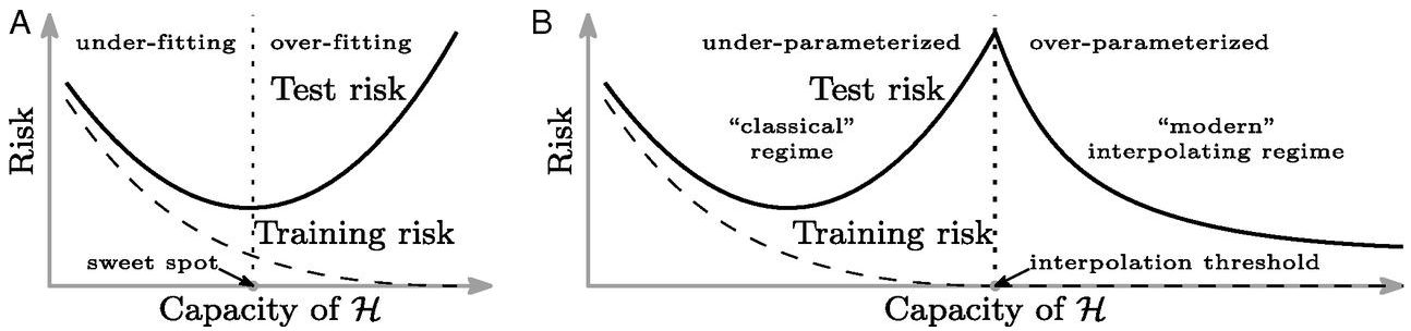
Figure: Left traditional perspective on generalization. There is a sweet spot of operation where the training error is still non-zero. Overfitting occurs when the variance increases. Right The double descent phenomenon, the modern models operate in an interpolation regime where they reconstruct the training data fully but are well regularized in their interpolations for test data. Figure from Belkin et al. (2019).

But the modern empirical finding is that when we move beyond Daddy bear, into the dark forest of the massively overparameterized model we can achieve good generalization. Indeed, recent work is showing that large language models are even memorizing data (Carlini et al., 2020) like non-parametric models do.

As Zhang et al. (2017) starkly illustrated with their random labels experiment, within the dark forest there are some terrible places, big bad wolves of overfitting that will gobble up your model. But as empirical evidence shows there is also a safe and hospitable Grandma’s house where these highly overparameterized models are safely consumed. Fundamentally, it must be about the route you take through the forest, and the precautions you take to ensure the wolf doesn’t see where you’re going and beat you to the door.

There are two implications of this empirical result. Firstly, that there is a great deal of new theory that needs to be developed. Secondly, that theory is now obliged to conflate two aspects to modelling that we generally like to keep separate: the model and the algorithm.

Classical statistical theory around predictive generalization focusses specifically on the class of models that is being used for data fitting. Historically, whether that theory follows a Fisher-aligned estimation approach (see e.g., Vapnik (1998)) or model-based Bayesian approach (see e.g., Ghahramani (2015)), neither is fully equipped to deal with these new circumstances because, to continue our rather tortured analogy, these theories provide us with a characterization of the destination of the algorithm, and seek to ensure that we reach that destination. Modern machine learning requires theories of the journey and what our route through the forest should be.

Crucially, the destination is always associated with 100% accuracy on the training set. An objective that is always achievable for the overparameterized model.

Intuitively, it seems that a highly overparameterized model places Grandma’s house on the edge of the dark forest. Making it easily and quickly accessible to the algorithm. The larger the model, the more exposed Grandma’s house becomes. Perhaps this is due to some form of blessing of dimensionality brings Grandma’s house closer to the edge of the forest in a high dimensional setting. Really, we should think of Grandma’s house as a low dimensional manifold of destinations that are safe. A path through the forest where the wolf of overfitting doesn’t venture. In the GLM case, we know already that when the number of parameters matches the number of data there is precisely one location in parameter space where accuracy on the training data is 100%. Our previous misunderstanding of generalization stemmed from the fact that (seemingly) it is highly unlikely that this single point is a good place to be from the perspective of generalization. Additionally, it is often difficult to find. Finding the precise polynomial coefficients in a least squares regression to exactly fit the basis to a small data set such as the Olympic marathon data requires careful consideration of the numerical properties and an orthogonalization of the design matrix (Lawson and Hanson, 1995).

It seems that with a highly overparameterized model, these locations become easier to find and they provide good generalization properties. In machine learning this is known as the “double descent phenomenon” (see e.g., Belkin et al. (2019)).

Diagram from (Nakkiran-deepdouble19?)

See also this talk by Misha Belkin: http://www.ipam.ucla.edu/abstract/?tid=15552&pcode=GLWS4 and these related papers https://www.pnas.org/content/116/32/15849.short, https://www.pnas.org/content/117/20/10625

Neural Tangent Kernel

Another approach to analysis exploits the fact that optimization is occurring in a very high dimensional parameter space. By considering initializations that involve small random weights (known as the NTK initialization) and noting that small updates in the learning mean that the model doesn’t move far from this initialization (Jacot et al., 2018).

For very wide neural networks, when these conditions are fulfilled, the network can be approximately represented by a kernel known as the neural tangent kernel. A kernel is a regularizer that operates in function space rather than feature space.

Regularization in Optimization

Another interesting theoretical direction is to study the path that neural network algorithms take when finding the optima. For certain simple linear systems, you can analytically study the ‘gradient flow.’

Neural networks are normally trained by (stochastic) gradient descent. This is a discrete optimization algorithm where at each point, a step in the direction of the (approximate) gradient is taken.

Gradient flow replaces this discrete update with a differential equation, where the step at any point is an exact gradient update. As a result, the path of the optimization can be studied as a differential equation.

By making assumptions about the initialization, the optimum that gradient flow will find can be characterised. For a highly overparameterized linear model, Gunasekar et al. (2017) show in matrix factorization, that for particular initializations, the optimum will be a global optimum of the objective that minimizes the L2-norm.

By reparameterizing the linear model so that each \(w_i = u_i^2 - v_i^2\) and optimising in the space defined by \(\mathbf{u}\) and \(\mathbf{v}\) Woodworth et al. (2020) show that the L1 norm is found.

Other papers have looked at deep linear models (Arora et al., 2019) where \[ f(\mathbf{ x}; \mathbf{W}) = \mathbf{W}_4 \mathbf{W}_3 \mathbf{W}_2 \mathbf{W}_1 \mathbf{ x}. \] In these models, a gradient flow analysis shows that the model finds solutions where the linear mapping, \[ \mathbf{W}= \mathbf{W}_4 \mathbf{W}_3 \mathbf{W}_2 \mathbf{W}_1 \] is very low rank. This is highly suggestive of another type of regularization that could be occurring in deep neural networks. Low rank parameter matrices mean that the effective capacity of the neural network is reduced. Indeed, empirical observations of the rank of deep nets trained on data suggest that they may be finding such solutions.

Practical Optimisation Notes

Further Reading

Example: calculating a Hessian

\[ H(\mathbb{w}) = \frac{\text{d}^2}{\text{d}\mathbf{ w}\text{d}\mathbf{ w}^\top} L(\mathbf{ w}) := \frac{\text{d}}{\text{d}\mathbf{ w}} \mathbf{g}(\mathbf{ w}) \]

Efficient strategy: compute \(\mathbf{g}(\mathbf{ w})\) with reverse-mode, then apply forward-mode to obtain Hessian columns or HVPs (reverse-over-forward). Framework helpers: JAX jax.jacfwd(jax.jacrev(f)), PyTorch autograd.functional.hessian (memory heavy for large models).

Example: Hessian-vector product

\[ \mathbf{v}^\top H(\mathbf{ w}) = \frac{\text{d}}{\text{d}\mathbf{ w}} \left( \mathbf{v}^\top \mathbf{g}(\mathbf{ w}) \right) \]

Live-coding HVP in PyTorch (mixed-mode via backward-over-backward or autograd.functional). Using a quadratic ensures a non-zero Hessian (2I):

import torch as th
def f(w):
    return (w**2).sum()  # toy scalar loss; Hessian = 2I
w = th.randn(5, requires_grad=True)
g, = th.autograd.grad(f(w), w, create_graph=True)  # gradient with graph
v = th.randn_like(w)
hv, = th.autograd.grad(g, w, grad_outputs=v)  # Hessian-vector product = 2*v
hv

Further Reading

• Chapter 8 of Bishop-deeplearning24

Thanks!

For more information on these subjects and more you might want to check the following resources.

• company: Trent AI
• book: The Atomic Human
• twitter: @lawrennd
• podcast: The Talking Machines
• newspaper: Guardian Profile Page
• blog: http://inverseprobability.com

References