Deep Architectures

Review

• Advanced Data Science
• ML and the Physical World
• Deep Neural Networks

Basis Functions to Neural Networks

From Basis Functions to Neural Networks

• So far: linear models or “shallow learning”
• Consider instead function composition or “deep learning”

Neural Network Prediction Function

\[ f(\mathbf{ x}; \mathbf{W}) = \mathbf{ w}_4 ^\top\phi\left(\mathbf{W}_3 \phi\left(\mathbf{W}_2\phi\left(\mathbf{W}_1 \mathbf{ x}\right)\right)\right). \]

Linear Models as Basis + Weights

\[ f(\mathbf{ x}_i) = \mathbf{ w}^\top \boldsymbol{ \phi}(\mathbf{ x}_i). \]

Deep Neural Network

Deep Neural Network

Mathematically

\[ \begin{align*} \mathbf{ h}_{1} &= \phi\left(\mathbf{W}_1 \mathbf{ x}\right)\\ \mathbf{ h}_{2} &= \phi\left(\mathbf{W}_2\mathbf{ h}_{1}\right)\\ \mathbf{ h}_{3} &= \phi\left(\mathbf{W}_3 \mathbf{ h}_{2}\right)\\ f&= \mathbf{ w}_4 ^\top\mathbf{ h}_{3} \end{align*} \]

From Shallow to Deep

\[ f(\mathbf{ x}; \mathbf{W}) = \mathbf{ w}_4 ^\top\phi\left(\mathbf{W}_3 \phi\left(\mathbf{W}_2\phi\left(\mathbf{W}_1 \mathbf{ x}\right)\right)\right). \]

Gradient-based optimization

\[ E(\mathbf{W}) = \sum_{i=1}^nE(\mathbf{ y}_i, f(\mathbf{ x}_i; \mathbf{W})) \]

\[ \mathbf{W}_{t+1} = \mathbf{W}_t - \eta \nabla_\mathbf{W}E(\mathbf{W}) \]

Basic Multilayer Perceptron

\[ \small f_L(\mathbf{ x}) = \boldsymbol{ \phi}\left(\mathbf{b}_L+ \mathbf{W}_L\boldsymbol{ \phi}\left(\mathbf{b}_{L-1} + \mathbf{W}_{L-1} \boldsymbol{ \phi}\left( \cdots \boldsymbol{ \phi}\left(\mathbf{b}_1 + \mathbf{W}_1 \mathbf{ x}\right) \cdots \right)\right)\right) \]

Recursive MLP Definition

\[\begin{align} f_\ell(\mathbf{ x}) &= \boldsymbol{ \phi}\left(\mathbf{W}_\ell f_{\ell-1}(\mathbf{ x}) + \mathbf{b}_\ell\right),\quad l=1,\dots,L\\ f_0(\mathbf{ x}) &= \mathbf{ x} \end{align}\]

Rectified Linear Unit

Shallow ReLU Networks

\[\begin{align} \mathbf{h}(x) &= \operatorname{ReLU}(\mathbf{w}_1 x - \mathbf{b}_1)\\ f(x) &= \mathbf{w}_2^{\top} \, \mathbf{h}(x) \end{align}\]

ReLU Activations

Decision Boundaries

Decision Boundaries

Complexity (1D): number of kinks \(\propto\) width of network.

Depth vs Width: Representation Power

• Single hidden layer: number of kinks \(\approx O(\text{width})\)
• Deep ReLU networks: kinks \(\approx O(2^{\text{depth}})\)

Sawtooth Construction

\[\begin{align} f_l(x) &= 2\vert f_{l-1}(x)\vert - 2, \quad f_0(x) = x\\ f_l(x) &= 2 \operatorname{ReLU}(f_{l-1}(x)) + 2 \operatorname{ReLU}(-f_{l-1}(x)) - 2 \end{align}\]

Complexity (1D): number of kinks \(\approx O(2^{\text{depth}})\).

Higher-dimensional Geometry

• Regions: piecewise-linear, often triangular/polygonal in 2D
• Continuity arises despite stitching flat regions
• Early layers: few regions; later layers: many more

Chain Rule and Back Propgation

Historical Context

• 1957: Rosenblatt’s Perceptron with multiple layers
• Association units: deep structure with random weights
• Modern approach: adjust weights to minimise error

Parameterised Basis Functions

• Basis functions: \(\boldsymbol{ \phi}(\mathbf{ x}; \mathbf{V})\)
• Adjustable parameters: \(\mathbf{V}\) can be optimized
• Non-linear models: in both inputs and parameters

The Gradient Problem

• Model: \(f(\mathbf{ x}_i) = \mathbf{ w}^\top \boldsymbol{ \phi}(\mathbf{ x}_i; \mathbf{V})\)
• Easy gradient: \(\frac{\text{d}f_i}{\text{d}\mathbf{ w}} = \boldsymbol{ \phi}(\mathbf{ x}_i; \mathbf{V})\)
• Hard gradient: \(\frac{\text{d}f_i}{\text{d}\mathbf{V}}\)

Chain Rule Application

\[\frac{\text{d}f_i}{\text{d}\mathbf{V}} = \frac{\text{d}f_i}{\text{d}\boldsymbol{ \phi}_i}\frac{\text{d}\boldsymbol{ \phi}_i}{\text{d} \mathbf{V}}\]

The Matrix Challenge

• Chain rule: standard approach
• New challenge: \(\frac{\text{d}\boldsymbol{ \phi}_i}{\text{d} \mathbf{V}}\)
• Problem: derivative of vector with respect to matrix

Matrix Vector Chain Rule

Matrix Calculus Standards

• Multiple approaches to multivariate chain rule
• Mike Brookes’ method: preferred approach
• Reference: Brookes (2005)

Brookes’ Approach

• Never compute matrix derivatives directly
• Stacking operation: intermediate step
• Vector derivatives: easier to handle

Matrix Stacking

• Input: matrix \(\mathbf{A}\)
• Output: vector \(\mathbf{a}\)
• Process: stack columns vertically

Stacking Formula

\[\mathbf{a} = \begin{bmatrix} \mathbf{a}_{:, 1}\\ \mathbf{a}_{:, 2}\\ \vdots\\ \mathbf{a}_{:, q} \end{bmatrix}\]

• Column stacking: each column becomes a block
• Order: first column at top, last at bottom
• Size: \(mn \times 1\) vector from \(m \times n\) matrix

Vector Derivatives

\[\frac{\text{d} \mathbf{a}}{\text{d} \mathbf{b}} \in \Re^{m \times n}\]

• Input: \(\mathbf{a} \in \Re^{m \times 1}\), \(\mathbf{b} \in \Re^{n \times 1}\)
• Output: \(m \times n\) matrix
• Standard form: vector-to-vector derivatives

Matrix Stacking Notation

• \(\mathbf{C}\!:\) vector formed from matrix \(\mathbf{C}\)
• Stacking: columns of \(\mathbf{C}\) → \(\Re^{mn \times 1}\) vector
• Condition: \(\mathbf{C} \in \Re^{m \times n}\)

Matrix-Matrix Derivatives

\[\frac{\text{d} \mathbf{E}}{\text{d} \mathbf{C}} \in \Re^{pq \times mn}\]

• Input: \(\mathbf{E} \in \Re^{p \times q}\), \(\mathbf{C} \in \Re^{m \times n}\)
• Output: \(pq \times mn\) matrix
• Advantage: easier chain rule application

Kronecker Products

• Notation: \(\mathbf{F} \otimes \mathbf{G}\)
• Essential tool: for matrix derivatives
• Key role: in chain rule applications

Kronecker Products

• Notation: \(\mathbf{A} \otimes \mathbf{B}\)
• Input: matrices \(\mathbf{A} \in \Re^{m \times n}\), \(\mathbf{B} \in \Re^{p \times q}\)
• Output: \((mp) \times (nq)\) matrix

Visual Examples

Kronecker Product Visualization

Column vs Row Stacking

• Column stacking: \(\mathbf{I} \otimes \mathbf{K}\) - time independence
• Row stacking: \(\mathbf{K} \otimes \mathbf{I}\) - dimension independence
  
• Different structure: affects which variables are correlated

Kronecker Product Formula

\[(\mathbf{A} \otimes \mathbf{B})_{ij} = a_{i_1 j_1} b_{i_2 j_2}\]

• Index mapping: \(i = (i_1-1)p + i_2\), \(j = (j_1-1)q + j_2\)
• Block structure: each element of \(\mathbf{A}\) scaled by \(\mathbf{B}\)
• Size: \((mp) \times (nq)\) result

Basic Properties

• Distributive: \((\mathbf{A} + \mathbf{B}) \otimes \mathbf{C} = \mathbf{A} \otimes \mathbf{C} + \mathbf{B} \otimes \mathbf{C}\)
• Associative: \((\mathbf{A} \otimes \mathbf{B}) \otimes \mathbf{C} = \mathbf{A} \otimes (\mathbf{B} \otimes \mathbf{C})\)
• Mixed product: \((\mathbf{A} \otimes \mathbf{B})(\mathbf{C} \otimes \mathbf{D}) = \mathbf{A}\mathbf{C} \otimes \mathbf{B}\mathbf{D}\)

Identity and Zero

• Identity: \(\mathbf{I}_m \otimes \mathbf{I}_n = \mathbf{I}_{mn}\)
• Zero: \(\mathbf{0} \otimes \mathbf{A} = \mathbf{A} \otimes \mathbf{0} = \mathbf{0}\)
• Scalar: \(c \otimes \mathbf{A} = \mathbf{A} \otimes c = c\mathbf{A}\)

Transpose and Inverse

• Transpose: \((\mathbf{A} \otimes \mathbf{B})^\top = \mathbf{A}^\top \otimes \mathbf{B}^\top\)
• Inverse: \((\mathbf{A} \otimes \mathbf{B})^{-1} = \mathbf{A}^{-1} \otimes \mathbf{B}^{-1}\) (when both exist)
• Determinant: \(\det(\mathbf{A} \otimes \mathbf{B}) = \det(\mathbf{A})^q \det(\mathbf{B})^m\)

Matrix Stacking and Kronecker Products

Column Stacking

• Stacking: place columns of matrix on top of each other
• Notation: \(\mathbf{a} = \text{vec}(\mathbf{A})\) or \(\mathbf{a} = \mathbf{A}\!:\)
• Kronecker form: \(\mathbf{I} \otimes \mathbf{K}\) for column-wise structure

Row Stacking

• Alternative: stack rows instead of columns
• Kronecker form: \(\mathbf{K} \otimes \mathbf{I}\) for row-wise structure
• Different structure: changes which variables are independent

Computational Advantages

Efficient Matrix Operations

• Inversion: \((\mathbf{A} \otimes \mathbf{B})^{-1} = \mathbf{A}^{-1} \otimes \mathbf{B}^{-1}\)
• Eigenvalues: \(\lambda_i(\mathbf{A} \otimes \mathbf{B}) = \lambda_j(\mathbf{A}) \lambda_k(\mathbf{B})\)
• Determinant: \(\det(\mathbf{A} \otimes \mathbf{B}) = \det(\mathbf{A})^q \det(\mathbf{B})^m\)

Memory and Speed Benefits

• Storage: avoid storing full covariance matrix
• Operations: work with smaller component matrices
• Scaling: \(O(n^3)\) becomes \(O(n_1^3 + n_2^3)\) for \(n = n_1 n_2\)

Kronecker Product Simplification

\[(\mathbf{E}:)^{\top} \mathbf{F} \otimes \mathbf{G}=\left(\left(\mathbf{G}^{\top} \mathbf{E F}\right):\right)^{\top}\]

• Removal rule: Kronecker products often simplified
• Chain rule: typically produces this form
• Key insight: avoid direct Kronecker computation

Chain Rule Application

\[\frac{\text{d} E}{\text{d} \mathbf{H}:} \frac{\text{d} \mathbf{H}:}{\text{d} \mathbf{J}:}=\frac{\text{d} E}{\text{d} \mathbf{J}:}\]

\[\frac{\text{d}\mathbf{H}}{\text{d} \mathbf{J}} = \mathbf{F} \otimes \mathbf{G}\]

Kronecker Product Identities

\[\mathbf{F}^{\top} \otimes \mathbf{G}^{\top}=(\mathbf{F} \otimes \mathbf{G})^{\top}\]

\[(\mathbf{E} \otimes \mathbf{G})(\mathbf{F} \otimes \mathbf{H})=\mathbf{E F} \otimes \mathbf{G H}\]

Derivative Representations

• Two forms: row vector vs matrix
• Row vector: easier computation
• Matrix: better summarization

\[\frac{\text{d} E}{\text{d} \mathbf{J}:}=\left(\left(\frac{\text{d} E}{\text{d} \mathbf{J}}\right):\right)^{\top}\]

Useful Multivariate Derivatives

Derivative of $mathbf{A} wrt \(\mathbf{A}\)

• Problem: \(\mathbf{b} = \mathbf{A}\mathbf{x}\), find \(\frac{\text{d}\mathbf{b}}{\text{d}\mathbf{A}}\)
• Approach: indirect derivation via \(\mathbf{a}^\prime\)
• Key insight: stacking rows vs columns

Indirect Approach

\[\frac{\text{d}}{\text{d} \mathbf{a^\prime}} \mathbf{A} \mathbf{x}\]

• Size: \(m \times mn\) matrix
• Definition: \(\mathbf{a}^\prime = \left(\mathbf{A}^\top\right):\)
• Stacking: columns of \(\mathbf{A}^\top\) = rows of \(\mathbf{A}\)

Row-wise Structure

\[\mathbf{A}\mathbf{x} = \begin{bmatrix} \mathbf{a}_{1, :}^\top \mathbf{x} \\ \mathbf{a}_{2, :}^\top \mathbf{x} \\ \vdots \\ \mathbf{a}_{m, :}^\top \mathbf{x} \end{bmatrix}\]

• Structure: inner products of rows of \(\mathbf{A}\)
• Gradient: \(\frac{\text{d}\mathbf{a}_{i,:}^\top \mathbf{x}}{\text{d}\mathbf{a}_{i,:}} = \mathbf{x}\)
• Expectation: repeated versions of \(\mathbf{x}\)

Kronecker Product Tiling

\[\mathbf{I}_m \otimes \mathbf{x}^\top = \begin{bmatrix} \mathbf{x}^\top & \mathbf{0}& \cdots & \mathbf{0}\\ \mathbf{0}& \mathbf{x}^\top & \cdots & \mathbf{0}\\ \vdots & \vdots & \ddots & \vdots \\ \mathbf{0}& \mathbf{0}& \cdots& \mathbf{x}^\top \end{bmatrix}\]

• Pattern: tiling of \(\mathbf{x}^\top\)
• Size: \(m \times nm\) matrix
• Structure: \(\mathbf{x}\) repeated in blocks

Final Result

\[\frac{\text{d}}{\text{d} \mathbf{a^\prime}} \mathbf{A} \mathbf{x} = \mathbf{I}_{m} \otimes \mathbf{x}^\top\]

• Each row: derivative of \(b_i = \mathbf{a}_{i, :}^\top \mathbf{x}\)
• Non-zero elements: only where \(\mathbf{a}_{i, :}\) appears
• Values: \(\mathbf{x}\) in appropriate positions

Column Stacking Alternative

\[\frac{\text{d}}{\text{d} \mathbf{a}} \mathbf{A} \mathbf{x} = \mathbf{x}^\top \otimes \mathbf{I}_{m}\]

• Change: \(\mathbf{a} = \mathbf{A}:\) (column stacking)
• Method: reverse Kronecker product order
• Result: \(\mathbf{x}^\top \otimes \mathbf{I}_{m}\)

Column Stacking Structure

\[\mathbf{x}^\top \otimes \mathbf{I}_{m} = \begin{bmatrix} x_1 \mathbf{I}_m & x_2 \mathbf{I}_m & \cdots & x_n \mathbf{I}_m \end{bmatrix}\]

• Pattern: \(\mathbf{x}\) elements distributed across blocks
• Size: \(m \times mn\) matrix
• Correct: for column stacking of \(\mathbf{A}\)

Chain Rule for Neural Networks

Neural Network Chain Rule

• Goal: compute gradients for neural networks
• Approach: apply matrix derivative rules
• Key: three fundamental gradients needed

Neural Network Structure

\[\mathbf{ f}_\ell= \mathbf{W}_\ell\boldsymbol{ \phi}_{\ell-1}\]

\[\boldsymbol{ \phi}_{\ell} = \boldsymbol{ \phi}_{\ell}(\mathbf{ f}_{\ell})\]

• Activations: \(\mathbf{ f}_\ell\) at layer \(\ell\)
• Basis functions: applied to activations
• Weight matrix: \(\mathbf{W}_\ell\)

First and Final Layers

\[f_1 = \mathbf{W}_1 \mathbf{ x}\]

\[\mathbf{h} = \mathbf{h}(\mathbf{ f}_L)\]

• First layer: \(f_1 = \mathbf{W}_1 \mathbf{ x}\)
• Final layer: inverse link function
• Dummy basis: \(\mathbf{h} = \boldsymbol{ \phi}_L\)

Limitations

• Skip connections: not captured in this formalism
• Example: layer \(\ell-2\) → layer \(\ell\)
• Sufficient: for main aspects of deep network gradients

Three Fundamental Gradients

• Activation gradient: \(\frac{\text{d}\mathbf{ f}_\ell}{\text{d}\mathbf{ w}_\ell}\)
• Basis gradient: \(\frac{\text{d}\boldsymbol{ \phi}_{\ell}}{\text{d} \mathbf{ f}_{\ell}}\)
• Across-layer gradient: \(\frac{\text{d}\mathbf{ f}_\ell}{\text{d}\boldsymbol{ \phi}_{\ell-1}}\)

Activation Gradient

\[\frac{\text{d}\mathbf{ f}_\ell}{\text{d}\mathbf{ w}_\ell} = \boldsymbol{ \phi}_{\ell-1}^\top \otimes \mathbf{I}_{d_\ell}\]

• Size: \(d_\ell\times (d_{\ell-1} d)\)
• Input: \(\mathbf{ f}_\ell\) and \(\mathbf{ w}_\ell\)
• Kronecker product: key to the result

Basis Gradient

\[\frac{\text{d}\boldsymbol{ \phi}_{\ell}}{\text{d} \mathbf{ f}_{\ell}} = \boldsymbol{ \Phi}^\prime\]

\[\frac{\text{d}\phi_i^{(\ell)}(\mathbf{ f}_{\ell})}{\text{d} f_j^{(\ell)}}\]

• Size: \(d_\ell\times d_\ell\) matrix
• Elements: derivatives of basis functions
• Diagonal: if basis functions depend only on their own activations

Activations and Gradients

Across-Layer Gradient

\[\frac{\text{d}\mathbf{ f}_\ell}{\text{d}\boldsymbol{ \phi}_{\ell-1}} = \mathbf{W}_\ell\]

• Size: \(d_\ell\times d_{\ell-1}\)
• Matches: shape of \(\mathbf{W}_\ell\)
• Simple: just the weight matrix itself

Complete Chain Rule

\[\frac{\text{d} \mathbf{ f}_\ell}{\text{d}\mathbf{ w}_{\ell-k}} = \left[\prod_{i=0}^{k-1} \frac{\text{d} \mathbf{ f}_{\ell - i}}{\text{d} \boldsymbol{ \phi}_{\ell - i -1}}\frac{\text{d} \boldsymbol{ \phi}_{\ell - i -1}}{\text{d} \mathbf{ f}_{\ell - i -1}}\right] \frac{\text{d} \mathbf{ f}_{\ell-k}}{\text{d} \mathbf{ w}_{\ell - k}}\]

• Product: of all intermediate gradients
• Chain: from layer \(\ell\) back to layer \(\ell-k\)
• Complete: gradient computation for any layer

Substituted Matrix Form

\[\frac{\text{d} \mathbf{ f}_\ell}{\text{d}\mathbf{ w}_{\ell-k}} = \left[\prod_{i=0}^{k-1} \mathbf{W}_{\ell - i} \boldsymbol{ \Phi}^\prime_{\ell - i -1}\right] \boldsymbol{ \phi}_{\ell-k-1}^\top \otimes \mathbf{I}_{d_{\ell-k}}\]

• Weight matrices: \(\mathbf{W}_{\ell - i}\) for across-layer gradients
• Basis derivatives: \(\boldsymbol{ \Phi}^\prime_{\ell - i -1}\) for activation derivatives
• Final term: Kronecker product for activation gradient

Gradient Verification

Verify Neural Network Gradients

Loss Functions

Test loss function gradients

Simple Deep NN Implementation

}

Create and Test Neural Network

Test Backpopagation

Train Network for Regression

mlai.write_figure(“nn-regression-training-progress.svg,” directory=“./ml”) }

{<object class=“svgplot” data=“https://mlatcl.github.io/mlfc/./slides/diagrams//ml/nn-regression-trainng-progress.”svg" width=“50%” style=" ">}{Neural Network Training Progress for a regression model){nn-regression-training-progress}

Visualise Decision Boundary

Evaluating Derivatives

\[ \frac{\text{d} \mathbf{ f}_L}{\text{d} \mathbf{ w}} = \frac{\text{d} \mathbf{ f}_L}{\text{d} \mathbf{ f}_{L-1}} \frac{\text{d} \mathbf{ f}_{L-1}}{\text{d} \mathbf{ f}_{L-2}} \frac{\text{d} \mathbf{ f}_{L-2}}{\text{d} \mathbf{ f}_{L-3}} \cdots \frac{\text{d} \mathbf{ f}_3}{\text{d} \mathbf{ f}_{2}} \frac{\text{d} \mathbf{ f}_2}{\text{d} \mathbf{ f}_{1}} \frac{\text{d} \mathbf{ f}_1}{\text{d} \mathbf{ w}} \]

\[ \small \frac{\text{d} \mathbf{ f}_L}{\text{d} \mathbf{ w}} = \frac{\text{d} \mathbf{ f}_L}{\text{d} \mathbf{ f}_{L-1}} \left( \frac{\text{d} \mathbf{ f}_{L-1}}{\text{d} \mathbf{ f}_{L-2}} \left( \frac{\text{d} \mathbf{ f}_{L-2}}{\text{d} \mathbf{ f}_{L-3}} \cdots \left( \frac{\text{d} \mathbf{ f}_3}{\text{d} \mathbf{ f}_{2}} \left( \frac{\text{d} \mathbf{ f}_2}{\text{d} \mathbf{ f}_{1}} \frac{\text{d} \mathbf{ f}_1}{\text{d} \mathbf{ w}} \right) \right) \cdots \right) \right) \]

Or like this?

\[ \frac{\text{d} \mathbf{ f}_L}{\text{d} \mathbf{ w}} = \frac{\text{d} \mathbf{ f}_L}{\text{d} \mathbf{ f}_{L-1}} \frac{\text{d} \mathbf{ f}_{L-1}}{\text{d} \mathbf{ f}_{L-2}} \frac{\text{d} \mathbf{ f}_{L-2}}{\text{d} \mathbf{ f}_{L-3}} \cdots \frac{\text{d} \mathbf{ f}_3}{\text{d} \mathbf{ f}_{2}} \frac{\text{d} \mathbf{ f}_2}{\text{d} \mathbf{ f}_{1}} \frac{\text{d} \mathbf{ f}_1}{\text{d} \mathbf{ w}} \]

\[ \small \frac{\text{d} \mathbf{ f}_L}{\text{d} \mathbf{ w}} = \left( \left( \cdots \left( \left( \frac{\text{d} \mathbf{ f}_L}{\text{d} \mathbf{ f}_{L-1}} \frac{\text{d} \mathbf{ f}_{L-1}}{\text{d} \mathbf{ f}_{L-2}} \right) \frac{\text{d} \mathbf{ f}_{L-2}}{\text{d} \mathbf{ f}_{L-3}} \right) \cdots \frac{\text{d} \mathbf{ f}_3}{\text{d} \mathbf{ f}_{2}} \right) \frac{\text{d} \mathbf{ f}_2}{\text{d} \mathbf{ f}_{1}} \right) \frac{\text{d} \mathbf{ f}_1}{\text{d} \mathbf{ w}} \]

Or in a funky way?

\[ \frac{\text{d} \mathbf{ f}_L}{\text{d} \mathbf{ w}} = \frac{\text{d} \mathbf{ f}_L}{\text{d} \mathbf{ f}_{L-1}} \frac{\text{d} \mathbf{ f}_{L-1}}{\text{d} \mathbf{ f}_{L-2}} \frac{\text{d} \mathbf{ f}_{L-2}}{\text{d} \mathbf{ f}_{L-3}} \cdots \frac{\text{d} \mathbf{ f}_3}{\text{d} \mathbf{ f}_{2}} \frac{\text{d} \mathbf{ f}_2}{\text{d} \mathbf{ f}_{1}} \frac{\text{d} \mathbf{ f}_1}{\text{d} \mathbf{ w}} \]

\[ \small \frac{\text{d} \mathbf{ f}_L}{\text{d} \mathbf{ w}} = \frac{\text{d} \mathbf{ f}_L}{\text{d} \mathbf{ f}_{L-1}} \left( \left( \left( \frac{\text{d} \mathbf{ f}_{L-1}}{\text{d} \mathbf{ f}_{L-2}} \right) \frac{\text{d} \mathbf{ f}_{L-2}}{\text{d} \mathbf{ f}_{L-3}} \right) \left( \left( \cdots \frac{\text{d} \mathbf{ f}_3}{\text{d} \mathbf{ f}_{2}} \right) \frac{\text{d} \mathbf{ f}_2}{\text{d} \mathbf{ f}_{1}} \right) \right)\frac{\text{d} \mathbf{ f}_1}{\text{d} \mathbf{ w}} \]

Automatic differentiation

Forward-mode

\[ \small \frac{\text{d} \mathbf{ f}_L}{\text{d} \mathbf{ w}} = \frac{\text{d} \mathbf{ f}_L}{\text{d} \mathbf{ f}_{L-1}} \left( \frac{\text{d} \mathbf{ f}_{L-1}}{\text{d} \mathbf{ f}_{L-2}} \left( \frac{\text{d} \mathbf{ f}_{L-2}}{\text{d} \mathbf{ f}_{L-3}} \cdots \left( \frac{\text{d} \mathbf{ f}_3}{\text{d} \mathbf{ f}_{2}} \left( \frac{\text{d} \mathbf{ f}_2}{\text{d} \mathbf{ f}_{1}} \frac{\text{d} \mathbf{ f}_1}{\text{d} \mathbf{ w}} \right) \right) \cdots \right) \right) \]

Cost: \[ \small d_0 d_1 d_2 + d_0 d_2 d_3 + \ldots + d_0 d_{L-1} d_L= d_0 \sum_{\ell=2}^{L} d_\ell d_{\ell-1} \]

Automatic Differentiation

Reverse-mode

\[ \small \frac{\text{d} \mathbf{ f}_L}{\text{d} \mathbf{ w}} = \left( \left( \cdots \left( \left( \frac{\text{d} \mathbf{ f}_L}{\text{d} \mathbf{ f}_{L-1}} \frac{\text{d} \mathbf{ f}_{L-1}}{\text{d} \mathbf{ f}_{L-2}} \right) \frac{\text{d} \mathbf{ f}_{L-2}}{\text{d} \mathbf{ f}_{L-3}} \right) \cdots \frac{\text{d} \mathbf{ f}_3}{\text{d} \mathbf{ f}_{2}} \right) \frac{\text{d} \mathbf{ f}_2}{\text{d} \mathbf{ f}_{1}} \right) \frac{\text{d} \mathbf{ f}_1}{\text{d} \mathbf{ w}} \]

Cost: \[ \small d_Ld_{L-1}d_{L-2} + d_{L}d_{L-2} d_{L-3} + \ldots + d_Ld_{1} d_0 = d_L\sum_{\ell=0}^{L-2}d_\ell d_{\ell+1} \]

Memory cost of autodiff

Forward-mode

Store only:

• current activation \(\mathbf{ f}_l\) (\(d_l\))
• running JVP of size \(d_0 \times d_l\)
• current Jacobian \(d_l \times d_{l+1}\)

Reverse-mode

Cache activations \(\{\mathbf{ f}_l\}\) so local Jacobians can be applied during backward; higher memory than forward-mode.

Automatic differentiation

• in deep learning we’re most interested in scalar objectives
• \(d_L=1\), consequently, backward mode is always optimal
• in the context of neural networks this is backpropagation.
• backprop has higher memory cost than forwardprop

Backprop in deep networks

Autodiff: Practical Details

• Terminology: forward-mode = JVP; reverse-mode = VJP
• Non-scalar outputs: seed vector required (e.g. backward(grad_outputs))
• Stopping grads: .detach(), no_grad() in PyTorch

Autodiff: Practical Details

• Grad accumulation: .grad accumulates by default; call zero_grad()
• Memory: backprop caches intermediates; use checkpointing/rematerialisation
• Mixed-mode: combine forward+reverse for Hessian-vector products

Computational Graphs and PyTorch Autodiff

• Nodes: tensors and ops; Edges: data dependencies
• Forward pass caches intermediates needed for backward
• Backward pass applies local Jacobian-vector products

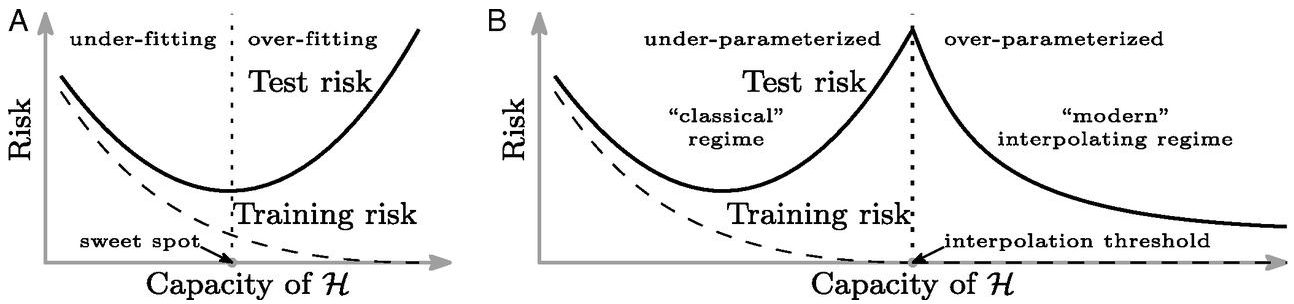
Overparameterised Systems

• Neural networks are highly overparameterised.
• If we could examine their Hessian at “optimum”
  • Very low (or negative) eigenvalues.
  • Error function is not sensitive to changes in parameters.
  • Implies parmeters are badly determined

Whence Generalisation?

• Not enough regularisation in our objective functions to explain.
• Neural network models are not using traditional generalisation approaches.
• The ability of these models to generalise must be coming somehow from the algorithm*
• How to explain it and control it is perhaps the most interesting theoretical question for neural networks.

Double Descent

Neural Tangent Kernel

• Consider very wide neural networks.
• Consider particular initialisation.
• Deep neural network is regularising with a particular kernel.
• This is known as the neural tangent kernel (Jacot et al., 2018).

Regularization in Optimization

• Gradient flow methods allow us to study nature of optima.
• In particular systems, with given initialisations, we can show L1 and L2 norms are minimised.
• In other cases the rank of \(\mathbf{W}\) is minimised.
• Questions remain over the nature of this regularisation in neural networks.

Deep Linear Models

\[ f(\mathbf{ x}; \mathbf{W}) = \mathbf{W}_4 \mathbf{W}_3 \mathbf{W}_2 \mathbf{W}_1 \mathbf{ x}. \]

\[ \mathbf{W}= \mathbf{W}_4 \mathbf{W}_3 \mathbf{W}_2 \mathbf{W}_1 \]

Practical Optimisation Notes

• Initialisation: variance-preserving (He, Xavier); scale affects signal propagation
• Optimisers: SGD(+momentum), Adam/AdamW; decoupled weight decay often preferable
• Learning rate schedules: cosine, step, warmup; LR is the most sensitive hyperparameter
• Batch size: affects gradient noise and implicit regularisation; tune with LR
• Normalisation: BatchNorm/LayerNorm stabilise optimisation
• Regularisation: data augmentation, dropout, weight decay; early stopping

Further Reading

• Baydin et al. (2018) Automatic differentiation in ML (JMLR)
• Jacot, Gabriel, Hongler (2018) Neural Tangent Kernel
• Arora et al. (2019) On exact dynamics of deep linear networks
• Keskar et al. (2017) Large-batch training and sharp minima
• Novak et al. (2018) Sensitivity and generalisation in neural networks
• JAX Autodiff Cookbook (JVPs/VJPs, jacfwd/jacrev)
• PyTorch Autograd Docs (computational graph, grad_fn, backward)

Example: calculating a Hessian

\[ H(\mathbb{w}) = \frac{\text{d}^2}{\text{d}\mathbf{ w}\text{d}\mathbf{ w}^\top} L(\mathbf{ w}) := \frac{\text{d}}{\text{d}\mathbf{ w}} \mathbf{g}(\mathbf{ w}) \]

Example: Hessian-vector product

\[ \mathbf{v}^\top H(\mathbf{ w}) = \frac{\text{d}}{\text{d}\mathbf{ w}} \left( \mathbf{v}^\top \mathbf{g}(\mathbf{ w}) \right) \]