Week 4: Latent Variables and Visualisation

[jupyter][google colab][reveal]

Neil D. Lawrence

Abstract:

This lecture introduces different approaches to discovering latent structure in data. We begin by examining clustering as a discrete approach to finding latent structure, then explore why high dimensional data often has simpler underlying continuous representations. This motivates our introduction to Principal Component Analysis (PCA) as a fundamental approach to continuous latent variable modeling.

ML Foundations Course Notebook Setup

We install some bespoke codes for creating and saving plots as well as loading data sets.

%%capture
%pip install notutils
%pip install git+https://github.com/lawrennd/ods.git
%pip install git+https://github.com/lawrennd/mlai.git

import notutils
import pods
import mlai
import mlai.plot as plot

High Dimensional Data

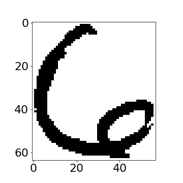
To introduce how to think about high dimensional data, we will first of all introduce a hand written digit from the U.S. Postal Service handwritten digit data set (originally collected from scanning enveolopes) and used in the first convolutional neural network paper (Le Cun et al., 1989).

Le Cun et al. (1989) downscaled the images to \(16 \times 16\), here we use an image at the original scale, containing 64 rows and 57 columns. Since the pixels are binary, and the number of dimensions is 3,648, this space contains \(2^{3,648}\) possible images. So this space contains a lot more than just one digit.

USPS Samples

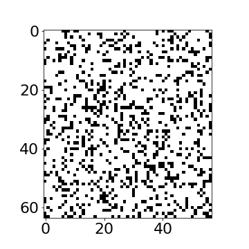
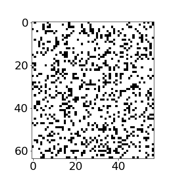
If we sample from this space, taking each pixel independently from a probability which is given by the number of pixels which are ‘on’ in the original image, over the total number of pixels, we see images that look nothing like the original digit.

Figure: Even if we sample every nano second from now until the end of the universe we won’t see the original six again.

Simple Model of Digit

An independent pixel model for this digit doesn’t seem sensible. The total space is enormous, and yet the space occupied by the type of data we’re interested in is relatively small.

Probability of Random Image Generation

Let’s consider a simple model for handwritten 6s. We model each pixel independently with a binomial distribution. Each pixel is the result of a single binomial trial, known as a Bernoulli distribution. \[ p(\mathbf{ y}) = \prod_{j=1}^d\pi^{y_j} (1-\pi)^{(1-y_j)}, \] where the probability across pixels are taken to be independent and are governed by the same probability of being on, \(\pi\). The maximum likelihood solution for this parameter is given by the number of pixels that are on in the data point divided by the total number of pixels \[ \pi= \frac{849}{3,648}. \] The probability of recovering the original six in any given sample is then given by \[ p(\mathbf{ y}=\text{given\,image}) = \pi^{849}(1-\pi)^{3,648 - 849 }=2.67\times10^{-860}. \]

This demonstrates why independent pixel models are inadequate for high-dimensional data. The probability of generating the original image by random sampling is so small (\(2.67 \times 10^{-860}\)) that it’s effectively impossible. This highlights the need for more sophisticated models that capture the underlying structure and dependencies in the data.

Consider a different type of model. One where we take a prototype six and we rotate it left and right to create new data.

%pip install scikit-image

from skimage.transform import rotate
import numpy as np
import mlai

# Load in the six
six_image = mlai.load_pgm('br1561_6.3.pgm', directory ='./ml')/255.0

# Pad out to 64 columns
rows = six_image.shape[0]
six_image = np.hstack([np.ones((rows, 3)), six_image, np.ones((rows, 4))])
dim_one = np.asarray(six_image.shape)
angles = range(360)
Y = np.zeros((len(angles), np.prod(dim_one)))
for i, angle in enumerate(angles):
    rot_image = rotate(six_image, angle, cval=1.0)
    dim_two = np.asarray(rot_image.shape)
    start = [int(round((dim_two[0] - dim_one[0])/2)), int(round((dim_two[1] - dim_one[1])/2))]
    crop_image = rot_image[start[0]+np.array(range(dim_one[0])), :][:, start[1]+np.array(range(dim_one[1]))]
    Y[i, :] = crop_image.flatten()

Figure: Rotate a prototype six to form a set of plausible sixes.

PCA of Rotated Sixes

Now let’s perform PCA on the rotated sixes to see how the data projects into a lower dimensional space. The rotated data should lie approximately on a one-dimensional manifold corresponding to the rotation angle.

import numpy as np

# Center the data
Y_centered = Y - np.mean(Y, axis=0)

# SVD of the centered data matrix (360 x 3648)
U, s, Vt = np.linalg.svd(Y_centered, full_matrices=False)

# Eigenvalues are s^2 / n 
eigenvalues = s**2 / Y.shape[0]

# Project data onto principal components
# Standard approach: X = U @ diag(s) gives the projections
X = U @ np.diag(s)

def plot_pca_manifold(X, Y, dims, filename, show_every=20, angle_ranges=None, colors=None):
    """Plot PCA manifold with optional angle range filtering"""
    fig, ax = plt.subplots(figsize=plot.big_figsize)
    h_points = ax.plot(X[:, 0], X[:, 1], 'rx', linewidth=2, alpha=0.7)[0]
    show_indices = range(0, len(X), show_every)  # Every 20 degrees
    if angle_ranges is None:
        # Plot all points
        show_indices = range(0, len(X), show_every)  # Every 20 degrees
    else:
        # Plot specific angle ranges
        h_points.set_data([], [])
        for i, (start, end, color) in enumerate(zip(angle_ranges['starts'], 
                                                   angle_ranges['ends'], 
                                                   colors or ['r', 'b'])):
            mask = (np.arange(len(X)) >= start) & (np.arange(len(X)) < end)
            ax.plot(X[mask, 0], X[mask, 1], f'{color}x', linewidth=2, alpha=0.7)
        
        # Show images only in specified ranges
        orig_show = show_indices
        show_indices = []
        for start, end in zip(angle_ranges['starts'], angle_ranges['ends']):
            for ind in orig_show:
                if ind >= start and ind <= end:
                    show_indices.append(ind)
    
    # Add small image insets
    for i in show_indices:
        if i < len(X):
            ax.scatter(X[i, 0], X[i, 1], s=50)
            
            # Calculate position for small image
            x_pos, y_pos = X[i, 0], X[i, 1]
            
            # Get plot limits and convert to figure coordinates
            x_min, x_max = ax.get_xlim()
            y_min, y_max = ax.get_ylim()
            
            x_fig = 0.1 + 0.8 * (x_pos - x_min) / (x_max - x_min)
            y_fig = 0.1 + 0.8 * (y_pos - y_min) / (y_max - y_min)
            
            inset_ax = fig.add_axes([x_fig, y_fig, 0.05, 0.05])
            rotated_img = Y[i, :].reshape(dims)
            inset_ax.imshow(rotated_img, cmap='gray')
            inset_ax.axis('off')
    
    ax.grid(True, alpha=0.3)
    
    mlai.write_figure(filename, directory='./dimred/')
    return fig, ax

Figure: The rotated sixes projected onto the first two principal components. The data lives on a one-dimensional manifold in the high-dimensional space, forming approximately a circle in the 2D projection.

Figure: The rotated sixes projected onto the first two principal components as sixes and nines. The six and nine data live on two separate one-dimensional manifolds in the high-dimensional space, forming two arcs from a circle in the 2D projection.

Interpoint Distances for Rotated Sixes

In this section we take all 360 examples of the rotated digits and analyze their interpoint distances. The data set is inherently one dimensional, with the dimension associated with the rotation transformation. A pure rotation would lead to a pure circle in the projected space. In practice, rotation of images requires some interpolation and this leads to small corruptions of the latent projections away from the circle.

# Calculate variance of each dimension
varY = np.var(Y, axis=0)
# Sort by variance in descending order
sorted_indices = np.argsort(varY)[::-1]
# Take top q dimensions (e.g., q=50 for dimensionality reduction)
q = 50
order = sorted_indices[:q]

# Calculate interpoint distances for selected dimensions
Y_selected = Y[:, order]
# Compute squared distances between all pairs
distMat = np.zeros((Y.shape[0], Y.shape[0]))
for i in range(Y.shape[0]):
    for j in range(Y.shape[0]):
        distMat[i, j] = np.sum((Y_selected[i, :] - Y_selected[j, :])**2) / q

# Calculate error term
e = 2 * np.sum(varY[sorted_indices[q:]]) / Y.shape[1]

Figure: Inter-point squared distances for the rotated digits data. Much of the data structure can be seen in the matrix. All points are ordered by angle of rotation. We can see that the distance between two points with similar angle of rotation is small (note in the upper right and lower left corners the low distances associated with 6s rotated by roughly 360 degrees and unrotated 6s).

Figure: Hisgogram of squared distances vs theory for the rotated sixes.

Low Dimensional Manifolds

Of course, in practice pure rotation of the image is too simple a model. Digits can undergo several distortions and retain their nature. For example, they can be scaled, they can go through translation, they can udnergo ‘thinning.’ But, for data with ‘structure’ we expect fewer of these distortions than the dimension of the data. This means we expect data to live on a lower dimensonal manifold. This implies that we should deal with high dimensional data by looking for a lower dimensional (non-linear) embedding.

Latent Variables

Latent means hidden, and hidden variables are simply unobservable variables. The idea of a latent variable is crucial to the concept of artificial intelligence, machine learning and experimental design. A latent variable could take many forms. We might observe a man walking along a road with a large bag of clothes and we might infer that the man is walking to the laundrette. Our observations are a highly complex data space, the response in our eyes is processed through our visual cortex, the combination of the individual’s limb movememnts and the direction they are walking in all conflate in our heads to cause us to infer that (perhaps) the individual is going to the laundrette. We don’t know that the man is walking to the laundrette, but we have a model of the world that suggests that it’s a likely outcome for the very complex data. In some ways the latent variable can be seen as a compression of this very complex scene. If I were writing a book, I might write that “A man tripped over whilst walking to the laundrette.” In the reader’s mind an image of a man, perhaps laden with dirty clothes, may occur. All these ideas come from our expectations of the world around us. We can make further inference about the man, some of it perhaps plausible others less so. The man may be going to the laundrette because his washing machine is broken, or because he doesn’t have a large enough flat to have a washing machine, or because he’s carrying a duvet, or because he doesn’t like ironing. All of these may increase in probability given our observation, but they are still latent variables. Unless we follow the man back to his appartment, or start making other enquirires about the man, we don’t know the true answer.

It’s clear that to do inference about any complex system we must include latent variables. Latent variables are extremely powerful. In robotics, they are used to represent the state of the robot. The state of the robot may include its position (in x, y coordinates) its speed, its direction of facing. How are these variables unknown to the robot? Well the robot only posesses sensors, it can make observations of the nearest object in a certain direction, and it may have a map of its environment. If we represent the state of the robot as its position on a map, it may be uncertain of that position. If you go walking or running in the hills around Sheffield, you can take a very high quality ordnance survey map with you. However, unless you are a really excellent orienteer, when you are far from any given landmark, you will probably be uncertain about your true position on the map. These states are also latent variables.

In statistical analysis of experiments you try to control for each aspect of the experiment, in particular by randomisation. So if I’m interested in the ability of a particular fertiliser to improve the yield of a particular plant I may design an experiment where I apply the fertilizer to some plants (the treatment group) and withold the fertilizer from others (the control group). I then test to see whether the yield from the treatment group is better (or worse) than the control group. I may find that I have an excellent yield for the treatment group. However, what if I’d (unknowlingly) planted all my treatment plants in a sunny part of the field, and all the control plants in a shady part of the field. That would also be a latent variable, in this case known as a confounder. In statistical experimental design randomisation is used to attempt to eliminate the correlated effects of these confounders: you aim to ensure that if these confounders do exist their effects are not correlated with treatment and contorl. This is known as a randomised control trial.

Greek philosophers worried a great deal about what was knowable and what was unknowable. Adherents of philosophical Skeptisism were inspired by the idea that since your senses sometimes give you contradictory information, they cannot be trusted, and in extreme cases they chose to ignore their senses. This is an acknowledgement that very often the true state of the world cannot be known with precision. Unfortunately, these philosophers didn’t have a good understanding of probability, so they were unable to encapsulate their ideas through a degree of belief.

We often use language to express the compression of a complex behavior or patterns in a simpler way, for example we talk about motives as a useful distallation for a perhaps very complex patter of behavior. In physics we use principles of causation and simple laws to describe the world around us. Such motives or underlying principles are difficult to observe directly, our conclusions about them emerge over a period of time by observing indirect consequences of the latent variables.

Epistemic uncertainty allows us to deal with these worries by associating our degree of belief about the state of the world with a probaiblity distribution. This core idea underpins state space modelling, probabilistic graphical models and the wider field of latent variable modelling. In this session we are going to explore the idea in a simple linear system and see how it relates to factor analysis and principal component analysis.

Your Personality

At the beginning of the 20th century there was a great deal of interest amoungst psychologists in formalizing patterns of thought. The approach they used became known as factor analysis. The principle is that we observe a potentially high dimensional vector of characteristics about an individual. To formalize this, social scientists designed questionaires. We can envisage many questions that we may ask, but the assumption is that underlying these questions there are only a few traits that dictate the behavior. These models are known as latent trait models and the analysis is sometimes known as factor analysis. The idea is that there are a few characteristic traits that we are looking to discern. These traits or factors can be extracted by assimilating the high dimensional characteristics of the individual into a few latent factors.

Factor Analysis Model

This causes us to consider a model as follows, if we are given a high dimensional vector of features (perhaps questionaire answers) associated with an individual, \(\mathbf{ y}\), we assume that these factors are actually generated from a low dimensional vector latent traits, or latent variables, which determine the personality. \[ \mathbf{ y}= \mathbf{f}(\mathbf{ z}) + \boldsymbol{ \epsilon}, \] where \(\mathbf{f}(\mathbf{ z})\) is a vector valued function that is dependent on the latent traits and \(\boldsymbol{ \epsilon}\) is some corrupting noise. For simplicity, we assume that the function is given by a linear relationship, \[ \mathbf{f}(\mathbf{ z}) = \mathbf{W}\mathbf{ z} \] where we have introduced a matrix \(\mathbf{W}\) that is sometimes referred to as the factor loadings but we also immediately see is related to our multivariate linear regression models from the . That is because our vector valued function is of the form

\[ \mathbf{f}(\mathbf{ z}) = \begin{bmatrix} f_1(\mathbf{ z}) \\ f_2(\mathbf{ z}) \\ \vdots \\ f_p(\mathbf{ z})\end{bmatrix} \] where there are \(d\) features associated with the individual. If we consider any of these functions individually we have a prediction function that looks like a regression model, \[ f_j(\mathbf{ z}) = \mathbf{ w}_{j, :}^\top \mathbf{ z}, \] for each element of the vector valued function, where \(\mathbf{ w}_{:, j}\) is the \(j\)th column of the matrix \(\mathbf{W}\). In that context each column of \(\mathbf{W}\) is a vector of regression weights. This is a multiple input and multiple output regression. Our inputs (or covariates) have dimensionality greater than 1 and our outputs (or response variables) also have dimensionality greater than one. Just as in a standard regression, we are assuming that we don’t observe the function directly (note that this also makes the function a type of latent variable), but we observe some corrupted variant of the function, where the corruption is given by \(\boldsymbol{ \epsilon}\). Just as in linear regression we can assume that this corruption is given by Gaussian noise, where the noise for the \(j\)th element of \(\mathbf{ y}\) is by, \[ \epsilon_j \sim \mathscr{N}\left(0,\sigma^2_j\right). \] Of course, just as in a regression problem we also need to make an assumption across the individual data points to form our full likelihood. Our data set now consists of many observations of \(\mathbf{ y}\) for diffetent individuals. We store these observations in a design matrix, \(\mathbf{Y}\), where each row of \(\mathbf{Y}\) contains the observation for one individual. To emphasize that \(\mathbf{ y}\) is a vector derived from a row of \(\mathbf{Y}\) we represent the observation of the features associated with the \(i\)th individual by \(\mathbf{ y}_{i, :}\), and place each individual in our data matrix, \[ \mathbf{Y} = \begin{bmatrix} \mathbf{ y}_{1, :}^\top \\ \mathbf{ y}_{2, :}^\top \\ \vdots \\ \mathbf{ y}_{n, :}^\top\end{bmatrix}, \] where we have \(n\) data points. Our data matrix therefore has \(n\) rows and \(p\) columns. The point to notice here is that each data obsesrvation appears as a row vector in the design matrix (thus the transpose operation inside the brackets). Our prediction functions are now actually a matrix value function, \[ \mathbf{F} = \mathbf{Z}\mathbf{W}^\top, \] where for each matrix the data points are in the rows and the data features are in the columns. This implies that if we have \(q\) inputs to the function we have \(\mathbf{F}\in \Re^{n\times p}\), \(\mathbf{W}\in \Re^{p \times q}\) and \(\mathbf{Z}\in \Re^{n\times q}\).

Exercise 1

Show that, given all the definitions above, if, \[ \mathbf{F} = \mathbf{Z}\mathbf{W}^\top \] and the elements of the vector valued function \(\mathbf{F}\) are given by \[ f_{i, j} = f_j(\mathbf{ z}_{i, :}), \] where \(\mathbf{ z}_{i, :}\) is the \(i\)th row of the latent variables, \(\mathbf{Z}\), then show that \[ f_j(\mathbf{ z}_{i, :}) = \mathbf{ w}_{j, :}^\top \mathbf{ z}_{i, :} \]

Latent Variables vs Linear Regression

The difference between this model and a multiple output regression is that in the regression case we are provided with the covariates \(\mathbf{Z}\), here they are latent variables. These variables are unknown. Just as we have done in the past for unknowns, we now treat them with a probability distribution. In factor analysis we assume that the latent variables have a Gaussian density which is independent across both across the latent variables associated with the different data points, and across those associated with different data features, so we have, \[ x_{i,j} \sim \mathscr{N}\left(0,1\right), \] and we can write the density governing the latent variable associated with a single point as, \[ \mathbf{ z}_{i, :} \sim \mathscr{N}\left(\mathbf{0},\mathbf{I}\right). \] If we consider the values of the function for the \(i\)th data point as \[ \mathbf{f}_{i, :} = \mathbf{f}(\mathbf{ z}_{i, :}) = \mathbf{W}\mathbf{ z}_{i, :} \] then we can use the rules for multivariate Gaussian relationships to write that \[ \mathbf{f}_{i, :} \sim \mathscr{N}\left(\mathbf{0},\mathbf{W}\mathbf{W}^\top\right) \] which implies that the distribution for \(\mathbf{ y}_{i, :}\) is given by \[ \mathbf{ y}_{i, :} = \sim \mathscr{N}\left(\mathbf{0},\mathbf{W}\mathbf{W}^\top + \boldsymbol{\Sigma}\right) \] where \(\boldsymbol{\Sigma}\) the covariance of the noise variable, \(\epsilon_{i, :}\) which for factor analysis is a diagonal matrix (because we have assumed that the noise was independent across the features), \[ \boldsymbol{\Sigma} = \begin{bmatrix}\sigma^2_{1} & 0 & 0 & 0\\ 0 & \sigma^2_{2} & 0 & 0\\ 0 & 0 & \ddots & 0\\ 0 & 0 & 0 & \sigma^2_p\end{bmatrix}. \] For completeness, we could also add in a mean for the data vector \(\boldsymbol{ \mu}\), \[ \mathbf{ y}_{i, :} = \mathbf{W}\mathbf{ z}_{i, :} + \boldsymbol{ \mu}+ \boldsymbol{ \epsilon}_{i, :} \] which would give our marginal distribution for \(\mathbf{ y}_{i, :}\) a mean \(\boldsymbol{ \mu}\). However, the maximum likelihood solution for \(\boldsymbol{ \mu}\) turns out to equal the empirical mean of the data, \[ \boldsymbol{ \mu}= \frac{1}{n} \sum_{i=1}^n \mathbf{ y}_{i, :}, \] regardless of the form of the covariance, \(\mathbf{C}= \mathbf{W}\mathbf{W}^\top + \boldsymbol{\Sigma}\). As a result it is very common to simply preprocess the data and ensure it is zero mean. We will follow that convention for this session.

The prior density over latent variables is independent, and the likelihood is independent, that means that the marginal likelihood here is also independent over the data points. Factor analysis was developed mainly in psychology and the social sciences for understanding personality and intelligence. Charles Spearman was concerned with the measurements of “the abilities of man” and is credited with the earliest version of factor analysis.

Principal Component Analysis

In 1933 Harold Hotelling published on principal component analysis the first mention of this approach (Hotelling, 1933). Hotelling’s inspiration was to provide mathematical foundation for factor analysis methods that were by then widely used within psychology and the social sciences. His model was a factor analysis model, but he considered the noiseless ‘limit’ of the model. In other words he took \(\sigma^2_i \rightarrow 0\) so that he had

\[ \mathbf{ y}_{i, :} \sim \lim_{\sigma^2 \rightarrow 0} \mathscr{N}\left(\mathbf{0},\mathbf{W}\mathbf{W}^\top + \sigma^2 \mathbf{I}\right). \] The paper had two unfortunate effects. Firstly, the resulting model is no longer valid probablistically, because the covariance of this Gaussian is ‘degenerate.’ Because \(\mathbf{W}\mathbf{W}^\top\) has rank of at most \(q\) where \(q<p\) (due to the dimensionality reduction) the determinant of the covariance is zero, meaning the inverse doesn’t exist so the density, \[ p(\mathbf{ y}_{i, :}|\mathbf{W}) = \lim_{\sigma^2 \rightarrow 0} \frac{1}{(2\pi)^\frac{p}{2} |\mathbf{W}\mathbf{W}^\top + \sigma^2 \mathbf{I}|^{\frac{1}{2}}} \exp\left(-\frac{1}{2}\mathbf{ y}_{i, :}\left[\mathbf{W}\mathbf{W}^\top+ \sigma^2 \mathbf{I}\right]^{-1}\mathbf{ y}_{i, :}\right), \] is not valid for \(q<p\) (where \(\mathbf{W}\in \Re^{p\times q}\)). This mathematical consequence is a probability density which has no ‘support’ in large regions of the space for \(\mathbf{ y}_{i, :}\). There are regions for which the probability of \(\mathbf{ y}_{i, :}\) is zero. These are any regions that lie off the hyperplane defined by mapping from \(\mathbf{ z}\) to \(\mathbf{ y}\) with the matrix \(\mathbf{W}\). In factor analysis the noise corruption, \(\boldsymbol{ \epsilon}\), allows for points to be found away from the hyperplane. In Hotelling’s PCA the noise variance is zero, so there is only support for points that fall precisely on the hyperplane. Secondly, Hotelling explicity chose to rename factor analysis as principal component analysis, arguing that the factors social scientist sought were different in nature to the concept of a mathematical factor. This was unfortunate because the factor loadings, \(\mathbf{W}\) can also be seen as factors in the mathematical sense because the model Hotelling defined is a Gaussian model with covariance given by \(\mathbf{C}= \mathbf{W}\mathbf{W}^\top\) so \(\mathbf{W}\) is a factor of the covariance in the mathematical sense, as well as a factor loading.

However, the paper had one great advantage over standard approaches to factor analysis. Despite the fact that the model was a special case that is subsumed by the more general approach of factor analysis it is this special case that leads to a particular algorithm, namely that the factor loadings (or principal components as Hotelling referred to them) are given by an eigenvalue decomposition of the empirical covariance matrix.

Computation of the Marginal Likelihood

\[ \mathbf{ y}_{i,:}=\mathbf{W}\mathbf{ z}_{i,:}+\boldsymbol{ \epsilon}_{i,:},\quad \mathbf{ z}_{i,:} \sim \mathscr{N}\left(\mathbf{0},\mathbf{I}\right), \quad \boldsymbol{ \epsilon}_{i,:} \sim \mathscr{N}\left(\mathbf{0},\sigma^{2}\mathbf{I}\right) \]

\[ \mathbf{W}\mathbf{ z}_{i,:} \sim \mathscr{N}\left(\mathbf{0},\mathbf{W}\mathbf{W}^\top\right) \]

\[ \mathbf{W}\mathbf{ z}_{i, :} + \boldsymbol{ \epsilon}_{i, :} \sim \mathscr{N}\left(\mathbf{0},\mathbf{W}\mathbf{W}^\top + \sigma^2 \mathbf{I}\right) \]

Probabilistic PCA Max. Likelihood Soln (Tipping and Bishop (1999a))

Figure: Graphical model representing probabilistic PCA.

\[p\left(\mathbf{Y}|\mathbf{W}\right)=\prod_{i=1}^{n}\mathscr{N}\left(\mathbf{ y}_{i, :}|\mathbf{0},\mathbf{W}\mathbf{W}^{\top}+\sigma^{2}\mathbf{I}\right)\]

Eigenvalue Decomposition

Eigenvalue problems are widespreads in physics and mathematics, they are often written as a matrix/vector equation but we prefer to write them as a full matrix equation. In an eigenvalue problem you are looking to find a matrix of eigenvectors, \(\mathbf{U}\) and a diagonal matrix of eigenvalues, \(\boldsymbol{\Lambda}\) that satisfy the matrix equation \[ \mathbf{A}\mathbf{U} = \mathbf{U}\boldsymbol{\Lambda}. \] where \(\mathbf{A}\) is your matrix of interest. This equation is not trivially solvable through matrix inverse because matrix multiplication is not commutative, so premultiplying by \(\mathbf{U}^{-1}\) gives \[ \mathbf{U}^{-1}\mathbf{A}\mathbf{U} = \boldsymbol{\Lambda}, \] where we remember that \(\boldsymbol{\Lambda}\) is a diagonal matrix, so the eigenvectors can be used to diagonalise the matrix. When performing the eigendecomposition on a Gaussian covariances, diagonalisation is very important because it returns the covariance to a form where there is no correlation between points.

Positive Definite

We are interested in the case where \(\mathbf{A}\) is a covariance matrix, which implies it is positive definite. A positive definite matrix is one for which the inner product, \[ \mathbf{ w}^\top \mathbf{C}\mathbf{ w} \] is positive for all values of the vector \(\mathbf{ w}\) other than the zero vector. One way of creating a positive definite matrix is to assume that the symmetric and positive definite matrix \(\mathbf{C}\in \Re^{p\times p}\) is factorised into, \(\mathbf{A}in \Re^{p\times p}\), a full rank matrix, so that \[ \mathbf{C}= \mathbf{A}^\top \mathbf{A}. \] This ensures that \(\mathbf{C}\) must be positive definite because \[ \mathbf{ w}^\top \mathbf{C}\mathbf{ w}=\mathbf{ w}^\top \mathbf{A}^\top\mathbf{A}\mathbf{ w} \] and if we now define a new vector \(\mathbf{b}\) as \[ \mathbf{b} = \mathbf{A}\mathbf{ w} \] we can now rewrite as \[ \mathbf{ w}^\top \mathbf{C}\mathbf{ w}= \mathbf{b}^\top\mathbf{b} = \sum_{i} b_i^2 \] which, since it is a sum of squares, is positive or zero. The constraint that \(\mathbf{A}\) must be full rank ensures that there is no vector \(\mathbf{ w}\), other than the zero vector, which causes the vector \(\mathbf{b}\) to be all zeros.

Exercise 2

If \(\mathbf{C}=\mathbf{A}^\top \mathbf{A}\) then express \(c_{i,j}\), the value of the element at the \(i\)th row and the \(j\)th column of \(\mathbf{C}\), in terms of the columns of \(\mathbf{A}\). Use this to show that (i) the matrix is symmetric and (ii) the matrix has positive elements along its diagonal.

Eigenvectors of a Symmetric Matric

Symmetric matrices have orthonormal eigenvectors. This means that \(\mathbf{U}\) is an orthogonal matrix, \(\mathbf{U}^\top\mathbf{U} = \mathbf{I}\). This implies that \(\mathbf{u}_{:, i} ^\top \mathbf{u}_{:, j}\) is equal to 0 if \(i\neq j\) and 1 if \(i=j\).

Probabilistic PCA

This linear relationship between the observed data and the latent variables is at the heart of Hotelling’s original formulation of PCA. It explicitly models the idea that the observed high-dimensional data is generated from a lower-dimensional set of latent variables, with some added noise. This perspective aligns PCA more closely with factor analysis and highlights its nature as a latent variable model.

Probabilistic PCA (PPCA) provides a probabilistic interpretation of PCA by explicitly modeling the generative process that creates the observed data. The model assumes that each high-dimensional data point \(\mathbf{ y}_{i,:}\) is generated from a lower-dimensional latent variable \(\mathbf{ z}_{i,:}\) through a linear transformation with added Gaussian noise: \[ \mathbf{ y}_{i,:} = \mathbf{W}\mathbf{ z}_{i,:} + \boldsymbol{ \epsilon}_{i,:} \] where \(\boldsymbol{ \epsilon}_{i,:} \sim \mathscr{N}\left(\mathbf{0},\sigma^2\mathbf{I}\right)\) represents isotropic Gaussian noise. The model places a standard Gaussian prior over the latent variables: \[ p(\mathbf{ z}_{i,:}) = \mathscr{N}\left(\mathbf{ z}_{i,:}|\mathbf{0},\mathbf{I}\right) \] Given these assumptions, the conditional probability of observing a data point given its latent representation is: \[ p(\mathbf{ y}_{i,:}|\mathbf{ z}_{i,:},\mathbf{W}) = \mathscr{N}\left(\mathbf{ y}_{i,:}|\mathbf{W}\mathbf{ z}_{i,:},\sigma^2\mathbf{I}\right) \] By integrating out the latent variables, we obtain the marginal likelihood of the data: \[ p(\mathbf{ y}_{i,:}|\mathbf{W}) = \mathscr{N}\left(\mathbf{ y}_{i,:}|\mathbf{0},\mathbf{W}\mathbf{W}^{\top}+\sigma^{2}\mathbf{I}\right) \] This probabilistic formulation, developed by Tipping and Bishop (Tipping and Bishop, 1999a), provides a principled framework that not only recovers classical PCA as a special case when \(\sigma^2 \to 0\), but also enables extensions like handling missing data and mixture models.

Figure: Graphical model representing probabilistic PCA.

Probabilistic PCA

In 1997 Tipping and Bishop (Tipping and Bishop, 1999b) and Roweis (Roweis, n.d.) independently revisited Hotelling’s model and considered the case where the noise variance was finite, but shared across all output dimensons. Their model can be thought of as a factor analysis where \[ \boldsymbol{\Sigma} = \sigma^2 \mathbf{I}. \] This leads to a marginal likelihood of the form \[ p(\mathbf{Y}|\mathbf{W}, \sigma^2) = \prod_{i=1}^n\mathscr{N}\left(\mathbf{ y}_{i, :}|\mathbf{0},\mathbf{W}\mathbf{W}^\top + \sigma^2 \mathbf{I}\right) \] where the limit of \(\sigma^2\rightarrow 0\) is not taken. This defines a proper probabilistic model. Tippping and Bishop then went on to prove that the maximum likelihood solution of this model with respect to \(\mathbf{W}\) is given by an eigenvalue problem. In the probabilistic PCA case the eigenvalues and eigenvectors are given as follows. \[ \mathbf{W}= \mathbf{U}\mathbf{L} \mathbf{R}^\top \] where \(\mathbf{U}\) is the eigenvectors of the empirical covariance matrix \[ \mathbf{S}= \sum_{i=1}^n(\mathbf{ y}_{i, :} - \boldsymbol{ \mu})(\mathbf{ y}_{i,:} - \boldsymbol{ \mu})^\top, \] which can be written \(\mathbf{S}= \frac{1}{n} \mathbf{Y}^\top\mathbf{Y}\) if the data is zero mean. The matrix \(\mathbf{L}\) is diagonal and is dependent on the eigenvalues of \(\mathbf{S}\), \(\boldsymbol{\Lambda}\). If the \(i\)th diagonal element of this matrix is given by \(\lambda_i\) then the corresponding element of \(\mathbf{L}\) is \[ \ell_i = \sqrt{\lambda_i - \sigma^2} \] where \(\sigma^2\) is the noise variance. Note that if \(\sigma^2\) is larger than any particular eigenvalue, then that eigenvalue (along with its corresponding eigenvector) is discarded from the solution.

PPCA as Manifold Learning

Probabilistic PCA can be viewed as a simple manifold learning algorithm. It assumes that:

1. The data lies near a linear manifold (subspace) of the high-dimensional space
2. The deviation from this manifold is Gaussian noise
3. The intrinsic dimensionality is specified by the number of retained components

This view helps explain why PPCA works well when the manifold hypothesis holds and the manifold is approximately linear. When the manifold is nonlinear, we need more sophisticated methods like kernel PCA or neural network-based approaches.

Python Implementation of Probabilistic PCA

We will now implement this algorithm in python.

import numpy as np

from mlai import ppca_eig

ppca = ppca_eig

In practice we may not wish to compute the eigenvectors of the covariance matrix directly. This is because it requires us to estimate the covariance, which involves a sum of squares term, before estimating the eigenvectors. We can estimate the eigenvectors directly either through QR decomposition or singular value decomposition. We saw a similar issue arise when , where we also wished to avoid computation of \(\mathbf{Z}^\top\mathbf{Z}\) (or in the case of \(\boldsymbol{\Phi}^\top\boldsymbol{\Phi}\)).

Posterior for Principal Component Analysis

Under the latent variable model justification for principal component analysis, we are normally interested in inferring something about the latent variables given the data. This is the distribution, \[ p(\mathbf{ z}_{i, :} | \mathbf{ y}_{i, :}) \] for any given data point. Determining this density turns out to be very similar to the approach for determining the Bayesian posterior of \(\mathbf{ w}\) in Bayesian linear regression, only this time we place the prior density over \(\mathbf{ z}_{i, :}\) instead of \(\mathbf{ w}\). The posterior is proportional to the joint density as follows, \[ p(\mathbf{ z}_{i, :} | \mathbf{ y}_{i, :}) \propto p(\mathbf{ y}_{i, :}|\mathbf{W}, \mathbf{ z}_{i, :}, \sigma^2) p(\mathbf{ z}_{i, :}) \] And as in the Bayesian linear regression case we first consider the log posterior, \[ \log p(\mathbf{ z}_{i, :} | \mathbf{ y}_{i, :}) = \log p(\mathbf{ y}_{i, :}|\mathbf{W}, \mathbf{ z}_{i, :}, \sigma^2) + \log p(\mathbf{ z}_{i, :}) + \text{const} \] where the constant is not dependent on \(\mathbf{ z}\). As before we collect the quadratic terms in \(\mathbf{ z}_{i, :}\) and we assemble them into a Gaussian density over \(\mathbf{ z}\). \[ \log p(\mathbf{ z}_{i, :} | \mathbf{ y}_{i, :}) = -\frac{1}{2\sigma^2} (\mathbf{ y}_{i, :} - \mathbf{W}\mathbf{ z}_{i, :})^\top(\mathbf{ y}_{i, :} - \mathbf{W}\mathbf{ z}_{i, :}) - \frac{1}{2} \mathbf{ z}_{i, :}^\top \mathbf{ z}_{i, :} + \text{const} \]

Exercise 3

Multiply out the terms in the brackets. Then collect the quadratic term and the linear terms together. Show that the posterior has the form \[ \mathbf{ z}_{i, :} | \mathbf{W}\sim \mathscr{N}\left(\boldsymbol{ \mu}_x,\mathbf{C}_x\right) \] where \[ \mathbf{C}_x = \left(\sigma^{-2} \mathbf{W}^\top\mathbf{W}+ \mathbf{I}\right)^{-1} \] and \[ \boldsymbol{ \mu}_x = \mathbf{C}_x \sigma^{-2}\mathbf{W}^\top \mathbf{ y}_{i, :} \] Compare this to the posterior for the Bayesian linear regression from last week, do they have similar forms? What matches and what differs?

Python Implementation of the Posterior

Now let’s implement the system in code.

Exercise 4

Use the values for \(\mathbf{W}\) and \(\sigma^2\) you have computed, along with the data set \(\mathbf{Y}\) to compute the posterior density over \(\mathbf{Z}\). Write a function of the form

mu_x, C_x = posterior(Y, W, sigma2)

where mu_x and C_x are the posterior mean and posterior covariance for the given \(\mathbf{Y}\).

Don’t forget to subtract the mean of the data Y inside your function before computing the posterior: remember we assumed at the beginning of our analysis that the data had been centred (i.e. the mean was removed).

Numerically Stable and Efficient Version

Just as we saw for and computation of a matrix such as \(\mathbf{Y}^\top\mathbf{Y}\) (or its centred version) can be a bad idea in terms of loss of numerical accuracy. Fortunately, we can find the eigenvalues and eigenvectors of the matrix \(\mathbf{Y}^\top\mathbf{Y}\) without direct computation of the matrix. This can be done with the singular value decomposition. The singular value decompsition takes a matrix, \(\mathbf{Z}\) and represents it in the form, \[ \mathbf{Z} = \mathbf{U}\boldsymbol{\Lambda}\mathbf{V}^\top \] where \(\mathbf{U}\) is a matrix of orthogonal vectors in the columns, meaning \(\mathbf{U}^\top\mathbf{U} = \mathbf{I}\). It has the same number of rows and columns as \(\mathbf{Z}\). The matrices \(\mathbf{\Lambda}\) and \(\mathbf{V}\) are both square with dimensionality given by the number of columns of \(\mathbf{Z}\). The matrix \(\mathbf{\Lambda}\) is diagonal and \(\mathbf{V}\) is an orthogonal matrix so \(\mathbf{V}^\top\mathbf{V} = \mathbf{V}\mathbf{V}^\top = \mathbf{I}\). The eigenvalues of the matrix \(\mathbf{Y}^\top\mathbf{Y}\) are then given by the singular values of the matrix \(\mathbf{Y}^\top\) squared and the eigenvectors are given by \(\mathbf{U}\).

Solution for \(\mathbf{W}\)

Given the singular value decomposition of \(\mathbf{Y}\) then we have \[ \mathbf{W}= \mathbf{U}\mathbf{L}\mathbf{R}^\top \] where \(\mathbf{R}\) is an arbitrary rotation matrix. This implies that the posterior is given by \[ \mathbf{C}_x = \left[\sigma^{-2}\mathbf{R}\mathbf{L}^2\mathbf{R}^\top + \mathbf{I}\right]^{-1} \] because \(\mathbf{U}^\top \mathbf{U} = \mathbf{I}\). Since, by convention, we normally take \(\mathbf{R} = \mathbf{I}\) to ensure that the principal components are orthonormal we can write \[ \mathbf{C}_x = \left[\sigma^{-2}\mathbf{L}^2 + \mathbf{I}\right]^{-1} \] which implies that \(\mathbf{C}_x\) is actually diagonal with elements given by \[ c_i = \frac{\sigma^2}{\sigma^2 + \ell^2_i} \] and allows us to write \[ \boldsymbol{ \mu}_x = [\mathbf{L}^2 + \sigma^2 \mathbf{I}]^{-1} \mathbf{L} \mathbf{U}^\top \mathbf{ y}_{i, :} \] \[ \boldsymbol{ \mu}_x = \mathbf{D}\mathbf{U}^\top \mathbf{ y}_{i, :} \] where \(\mathbf{D}\) is a diagonal matrix with diagonal elements given by \(d_{i} = \frac{\ell_i}{\sigma^2 + \ell_i^2}\).

import scipy as sp
import numpy as np

from mlai import ppca_svd

from mlai import ppca_posterior

ppca = ppca_svd
posterior = ppca_posterior

Scikit-learn implementation PCA

We’ve implemented PCA as part of supporting the learning process, but in practice we can use the scikit-learn implementation. Let’s try it on the oil flow data.

Oil Flow Data

This data set is from a physics-based simulation of oil flow in a pipeline. The data was generated as part of a project to determine the fraction of oil, water and gas in North Sea oil pipes (Bishop and James, 1993).

import pods

data = pods.datasets.oil()

The data consists of 1000 12-dimensional observations of simulated oil flow in a pipeline. Each observation is labelled according to the multi-phase flow configuration (homogeneous, annular or laminar).

# Convert data["Y"] from [1, -1, -1] in each row to rows of 0 or 1 or 2
Y = data["Y"]
# Find rows with 1 in first column (class 0)
class0 = (Y[:, 0] == 1).astype(int) * 0
# Find rows with 1 in second column (class 1) 
class1 = (Y[:, 1] == 1).astype(int) * 1
# Find rows with 1 in third column (class 2)
class2 = (Y[:, 2] == 1).astype(int) * 2
# Combine into single array of class labels 0,1,2
labels = class0 + class1 + class2

The data is returned as a dictionary containing training and test inputs (‘X,’ ‘Xtst’), training and test labels (‘Y,’ ‘Ytst’), and the names of the features.

Figure: Visualization of the first two dimensions of the oil flow data from Bishop and James (1993)

As normal we include the citation information for the data.

print(data['citation'])

And extra information about the data is included, as standard, under the keys info and details.

print(data['details'])

X = data['X']
Y = data['Y']

%pip install scikit-learn

from sklearn.decomposition import PCA

pca = PCA(n_components=2)
pca.fit(X)
X_pca = pca.transform(X)

# Find rows with 1 in first column (class 0)
class0 = (Y[:, 0] == 1).astype(int) * 0
# Find rows with 1 in second column (class 1) 
class1 = (Y[:, 1] == 1).astype(int) * 1
# Find rows with 1 in third column (class 2)
class2 = (Y[:, 2] == 1).astype(int) * 2
# Combine into single array of class labels 0,1,2
lbls = class0 + class1 + class2

Figure: PCA of the oil flow data. The flow is homogeneous, annular and stratified.

The Probabilistic PCA Model

For our notation, we express the \(i\)th data point’s position in the underlying latent space by the vector \(\mathbf{ z}_{i, :}\). The relationship between the latent space and the data space in the form of a linear mapping, [ {i, :} = {i, :} + + {i, :} ] where \(\mathbf{W}\in \Re^{d,q}\) is a mapping matrix which encodes the relationship between the latent space and the data space. The vector \(\boldsymbol{ \epsilon}\) represents the corrupting noise. We will assume the noise is independently sampled from a Gaussian density, [ {i,:} , ] where \(\sigma\) is the standard deviation of the corrupting noise.

Linear dimensionality reduction can be thought of as finding a lower dimensional plane embedded in a higher dimensional space. The plane is described by the matrix \(\mathbf{W}\). The direction of the vectors in this matrix define the orientation of the plane. The figure below shows how this works when the latent space is two dimensional and the data space is three dimensional.

Figure: Mapping a two dimensional plane to a higher dimensional space in a linear way. Data are generated by corrupting points on the plane with noise.

Examples: Motion Capture Data

OSU Motion Capture Data: Run 1

Motion capture data the Open Motion Data Project by The Ohio State University Advanced Computing Center for the Arts and Design. Historically the data website was found here http://accad.osu.edu/research/mocap/mocap_data.htm, although it is now missing. The centre website is here: https://accad.osu.edu.

import pods

You can download different data from the site, here we download the ‘run1’ motion.

data = pods.datasets.osu_run1()

The data dictionary contains the keys ‘Y’ and ‘connect,’ which represent the data and connections that can be used to create the skeleton.

data['Y'].shape

The data has often been used in talks demonstrating GP-LVM models and comparing variants such as back constrained and temporal models.

print(data['citation'])

And extra information about the data is included, as standard, under the keys under details.

print(data['details'])

Y = data['Y']

Once the data is loaded in we can examine the first two principal components as follows,

q = 2
U, ell, sigma2 = ppca(Y, q)
mu_x, C_x = posterior(Y, U, ell, sigma2)

Figure: First two principal components of motion capture data of an individual running.

Here because the data is a time course, we have connected points that are neighbouring in time. This highlights the form of the run, which involves 3 paces. This projects in our low dimensional space to 3 loops. We can examin how much residual variance there is in the system by looking at sigma2.

print(sigma2)

Robot Navigation Example

In the next example we will load in data from a robot navigation problem. The data consists of wireless access point strengths as recorded by a robot performing a loop around the University of Washington’s Computer Science department in Seattle. The robot records all the wireless access points it can cache and stores their signal strength.

import pods

data = pods.datasets.robot_wireless()
Y = data['Y']
Y.shape

There are 215 observations of 30 different access points. In this case the model is suggesting that the access point signal strength should be linearly dependent on the location in the map. In other words we are expecting the access point strength for the \(j\)th access point at robot position \(x_{i, :}\) to be represented by \(y_{i, j} = \mathbf{ w}_{j, :}^\top \mathbf{ z}_{i, :} + \epsilon_{i,j}\).

Figure: PCA of the robot wireless data.

Interpretations of Principal Component Analysis

Principal Component Analysis

Principal Component Analysis (PCA) is one of the most fundamental and widely used dimensionality reduction techniques. While commonly credited to Pearson (1901), who was interested in finding “lines and planes of closest fit to systems of points in space,” the method as we will review it today was introduced and named by Hotelling (Hotelling (1933)). The approach is often used as a way of looking for correlations, but Hotelling’s motivation was a principled alternative to Spearman’s factor analysis (Spearman, 1904).

Often PCA is introduced as a method for finding directions of maximum variance in high-dimensional data, and this is the interpretation that is due to Pearson (1901), but philosophically these approaches arre different even though they turn out to be identical mathematically. In a very real sense “many models lead to the PCA algorithm.” But these equivalences are only true when a linear interpretation is sought. Nonlinear extensions of these ideas (maximum variance directions, eigenvalue problems, latent variable models) all lead to different algorithms. However, since the linear algorithm has so many interpretations it is a wise place to begin analysis.

The mathematical foundation of PCA relies on analyzing the sample covariance matrix of the data. For a dataset with \(n\) points, this matrix is given by:

\[ \mathbf{S}=\frac{1}{n}\sum_{i=1}^n\left(\mathbf{ y}_{i, :}-\boldsymbol{ \mu}\right)\left(\mathbf{ y}_{i, :} - \boldsymbol{ \mu}\right)^\top \]

The modern interpretation focuses on finding a set of orthogonal directions (principal components) along which the data varies the most, but Hotelling’s original formulation was derived from the idea of latent variables. The optimization problem we solve today, which maximizes the variance along each direction while maintaining orthogonality constraints, arises as the solution of the original latent variable formulation (Tipping and Bishop, 1999a).

import numpy as np

# Generate correlated 2D Gaussian samples
num_points = 200
mean = np.array([0, 0])
cov = np.array([[2.0, 1.8], 
                [1.8, 2.0]])
X = np.random.multivariate_normal(mean, cov, num_points)

Figure: Illustration of PCA on 2D correlated Gaussian data. The arrows show the principal components (eigenvectors scaled by square root of eigenvalues). The ellipse represents the covariance structure.

Relationship to Matrix Factorization

We can use the robot naviation example to realise that PCA (and factor analysis) are very reminiscient of the that we used for introducing objective functions. In that system we used slightly different notation, \(\mathbf{u}_{i, :}\) for user location in our metaphorical library and \(\mathbf{v}_{j, :}\) for item location in our metaphorical library. To see how these systems are somewhat analagous, now let us think about the user as the robot and the items as the wifi access points. We can plot the relative location of both. This process is known as “SLAM”: simultaneous localisation and mapping. A latent variable model of the type we have developed is one way of performing SLAM. We have an estimate of the landmarks in the system (in this case WIFI access points) and we have an estimate of the robot position. These are analagous to the estimate of the user’s position and the estimate of the items positions in the library. In the matrix factorisation example users are informing us what items they are ‘close’ to by expressing their preferences, in the robot localization example the robot is informing us what access point it is close to by measuring signal strength.

From a personal perspective, I find this analogy quite comforting. I think it is very arguable that one of the mechanisms through which we (as humans) may have developed higher reasoning is through the need to navigate around our environment, identifying landmarks and associating them with our search for food. If such a system were to exist, the idea that it could be readily adapted to other domains such as categorising the nature of the different foodstuffs we were able to forage is intriguing.

From an algorithmic perspective, we also can now realise that matrix factorization and latent variable modelling are effectively the same thing. The only difference is the objective function and our probabilistic (or lack of probabilistic) treatment of the variables. But the prediction function for both systems, \[ f_{i, j} = \mathbf{u}_{i, :}^\top \mathbf{v}_{j, :} \] for matrix factorization or \[ f_{i, j} = \mathbf{ z}_{i, :}^\top \mathbf{ w}_{j, :} \] for probabilistic PCA and factor analysis are the same.

PCA: Separating Model and Algorithm

Since Hotelling first introduced his perspective on factor analysis as PCA there has been somewhat of a conflation of the idea of the model underlying PCA (for which it was very clear that Hotelling was inspired by Factor Analysis) and the algorithm that is used to fit that model: the eigenvalues and eigenvectors of the covariance matrix. The eigenvectors of an ellipsoid have been known since the middle of the 19th century as the principal axes of the elipsoid, and they arise through the following additional ideas: seeking the orthogonal directions of maximum variance in a dataset. Pearson in 1901 arrived at the same algorithm driven by a desire to seek a symmetric regression between two covariate/response variables \(x\) and \(y\) (Pearson:01?). He is, therefore, often credited with the invention of principal component analysis, but to me this seems disengenous. His aim was very different from Hotellings, it was just happened that the optimal solution for his model was coincident with that of Hotelling. The approach is also known as the Karhunen Loeve Transform in stochastic process theory and in classical multidimensional scaling the same operation can be shown to be minimising a particular objective function based on interpoint distances in the data and the latent space (see the section on Classical Multidimensional Scaling in Mardia, Kent and Bibby) (Mardia et al., 1979).

One of my own contributions to machine learning was deriving yet another model whose linear variant was solved by finding the principal subspace of the covariance matrix (an approach I termed dual probabilistic PCA or probabilistic principal coordinate analysis). Finally, the approach is sometimes referred to simply as singular value decomposition (SVD). The singular value decomposition of a data set has the following form, \[ \mathbf{Y}= \mathbf{V} \boldsymbol{\Lambda} \mathbf{U}^\top \] where \(\mathbf{V}\in\Re^{n\times n}\) and \(\mathbf{U}^\in \Re^{p\times p}\) are square orthogonal matrices and \(\mathbf{\Lambda}^{n \times p}\) is zero apart from its first \(p\) diagonal entries. Singularvalue decomposition gives a diagonalisation of the covariance matrix, because under the SVD we have \[ \mathbf{Y}^\top\mathbf{Y}= \mathbf{U}\boldsymbol{\Lambda}\mathbf{V}^\top\mathbf{V} \boldsymbol{\Lambda} \mathbf{U}^\top = \mathbf{U}\boldsymbol{\Lambda}^2 \mathbf{U}^\top \] where \(\boldsymbol{\Lambda}^2\) is now the eigenvalues of the covariane matrix and \(\mathbf{U}\) are the eigenvectors. So performing the SVD can simply be seen as another approach to determining the principal components.

Separating Model and Algorithm

I’ve given a fair amount of personal thought to this situation and my own opinion that this confusion about method arises because of a conflation of model and algorithm. The model of Hotelling, that which he termed principal component analysis, was really a variant of factor analysis, and it was unfortunate that he chose to rename it. However, the algorithm he derived was a very convenient way of optimising a (simplified) factor analysis, and it’s therefore become very popular. The algorithm is also the optimal solution for many other models of the data, even some which might seem initally to be unrelated (e.g. seeking directions of maximum variance). It is only through the mathematics of this linear system (which also contains some intersting symmetries) that all these ides become related. However, as soon as we choose to non-linearise the system (e.g. through basis functions) we find that each of the non-linear intepretations we can derive for the different models each leads to a very different algorithm (if such an algorithm is possible). For example principal curves of Hastie and Stuetzle (1989) attempt to non-linearise the maximum variance interpretation, kernel PCA of Schölkopf et al. (1998) uses basis functions to form the eigenvalue problem in a nonlinear space, and my own work in this area non-linearises the dual probabilistic PCA (Lawrence, 2005).

My conclusion is that when you are doing machine learning you should always have it clear in your mind what your model is and what your algorithm is. You can recognise your model because it normally contains a prediction function and an objective function. The algorithm on the other hand is the sequence of steps you implement on the computer to solve for the parameters of this model. For efficient implementation, we often modify our model to allow for faster algorithms, and this is a perfectly valid pragmatist’s approach, so conflation of model and algorithm is not always a bad thing. But for clarity of thinking and understanding it is necessary to maintain the separation and to maintain a handle on when and why we perform the conflation.

PCA Effectiveness

Principal component analysis is so effective in practice that there has almost developed a mini-industry in renaming the method itself (which is ironic, given its origin as a renaming of factor analysis). In particular Latent Semantic Indexing in text processing is simply PCA on a particular representation of the term frequencies of the document. There is a particular fad to rename the eigenvectors after the nature of the data you are examining, perhaps initially triggered by Turk and Pentland’s paper on eigenfaces, but also with eigenvoices and eigengenes.

This seems to be an instantiation of a wider, and hopefully subconcious, tendency in academia to attempt to differentiate one idea from the same idea in related fields in order to emphasise the novelty. The unfortunate result is somewhat of a confusing literature for relatively simple model.

My recommendations would be as follows. If you have multivariate data, applying some form of principal component would seem to be a very good idea as a first step. Even if you intend to later perform classification or regression on your data, it can give you understanding of the structure of the underlying data and help you to develop your intuitions about the nature of your data. Intelligent plotting and interaction with your data is always a good think, and for high dimensional data that means that you need some way of visualisation, PCA is typically a good starting point.

Indeed, sometimes I’ll say “have you done PCA yet?” is the data scientists equivalent of “have you switched it off and on again?”

Derivation of PPCA

PPCA Marginal Likelihood

We have developed the posterior density over the latent variables given the data and the parameters, and due to symmetries in the underlying prediction function, it has a very similar form to its sister density, the posterior of the weights given the data from Bayesian regression. Two key differences are as follows. If we were to do a Bayesian multiple output regression we would find that the marginal likelihood of the data is independent across the features and correlated across the data, \[ p(\mathbf{Y}|\mathbf{Z}) = \prod_{j=1}^d\mathscr{N}\left(\mathbf{ y}_{:, j}|\mathbf{0}, \alpha\mathbf{Z}\mathbf{Z}^\top + \sigma^2 \mathbf{I}\right) \] where \(\mathbf{ y}_{:, j}\) is a column of the data matrix and the independence is across the features, in probabilistic PCA the marginal likelihood has the form, \[ p(\mathbf{Y}|\mathbf{W}) = \prod_{i=1}^n\mathscr{N}\left(\mathbf{ y}_{i, :}|\mathbf{0},\mathbf{W}\mathbf{W}^\top + \sigma^2 \mathbf{I}\right) \] where \(\mathbf{ y}_{i, :}\) is a row of the data matrix \(\mathbf{Y}\) and the independence is across the data points.

Computation of the Log Likelihood

The quality of the model can be assessed using the log likelihood of this Gaussian form. \[ \log p(\mathbf{Y}|\mathbf{W}) = -\frac{n}{2} \log \left| \mathbf{W}\mathbf{W}^\top + \sigma^2 \mathbf{I}\right| -\frac{1}{2} \sum_{i=1}^n\mathbf{ y}_{i, :}^\top \left(\mathbf{W}\mathbf{W}^\top + \sigma^2 \mathbf{I}\right)^{-1} \mathbf{ y}_{i, :} +\text{const} \] but this can be computed more rapidly by exploiting the low rank form of the covariance covariance, \(\mathbf{C}= \mathbf{W}\mathbf{W}^\top + \sigma^2 \mathbf{I}\) and the fact that \(\mathbf{W}= \mathbf{U}\mathbf{L}\mathbf{R}^\top\).

Specifically, we first use the decomposition of \(\mathbf{W}\) to write \[ -\frac{n}{2} \log \left| \mathbf{W}\mathbf{W}^\top + \sigma^2 \mathbf{I}\right| = -\frac{n}{2} \sum_{i=1}^q\log (\ell_i^2 + \sigma^2) - \frac{n(d-q)}{2}\log \sigma^2, \] where \(\ell_i\) is the \(i\)th diagonal element of \(\mathbf{L}\).

Next, we use the Woodbury matrix identity which allows us to write the inverse as a quantity which contains another inverse in a smaller matrix \[ (\sigma^2 \mathbf{I}+ \mathbf{W}\mathbf{W}^\top)^{-1} = \sigma^{-2}\mathbf{I}-\sigma^{-4}\mathbf{W}{\underbrace{(\mathbf{I}+\sigma^{-2}\mathbf{W}^\top\mathbf{W})}_{\mathbf{C}_x}}^{-1}\mathbf{W}^\top \] So, it turns out that the original inversion of the \(d\times d\) matrix can be done by forming a quantity which contains the inversion of a \(q\times q\) matrix which, moreover, turns out to be the quantity \(\mathbf{C}_x\) of the posterior.

Now, we put everything together to obtain: \[ \log p(\mathbf{Y}|\mathbf{W}) = -\frac{n}{2} \sum_{i=1}^q \log (\ell_i^2 + \sigma^2) - \frac{n(d-q)}{2}\log \sigma^2 - \frac{1}{2} \text{tr}\left(\mathbf{Y}^\top \left( \sigma^{-2}\mathbf{I}-\sigma^{-4}\mathbf{W}\mathbf{C}_x \mathbf{W}^\top \right) \mathbf{Y}\right) + \text{const}, \] where we used the fact that a scalar sum can be written as \(\sum_{i=1}^n\mathbf{ y}_{i,:}^\top \mathbf{K}\mathbf{ y}_{i,:} = \text{tr}\left(\mathbf{Y}^\top \mathbf{K}\mathbf{Y}\right)\), for any matrix \(\mathbf{K}\) of appropriate dimensions. We now use the properties of the trace \(\text{tr}\left(\mathbf{A}+\mathbf{B}\right)=\text{tr}\left(\mathbf{A}\right)+\text{tr}\left(\mathbf{B}\right)\) and \(\text{tr}\left(c \mathbf{A}\right) = c \text{tr}\left(\mathbf{A}\right)\), where \(c\) is a scalar and \(\mathbf{A},\mathbf{B}\) matrices of compatible sizes. Therefore, the final log likelihood takes the form: \[ \log p(\mathbf{Y}|\mathbf{W}) = -\frac{n}{2} \sum_{i=1}^q\log (\ell_i^2 + \sigma^2) - \frac{n(d-q)}{2}\log \sigma^2 - \frac{\sigma^{-2}}{2} \text{tr}\left(\mathbf{Y}^\top \mathbf{Y}\right) +\frac{\sigma^{-4}}{2} \text{tr}\left(\mathbf{B}\mathbf{C}_x\mathbf{B}^\top\right) + \text{const} \] where we also defined \(\mathbf{B}=\mathbf{Y}^\top\mathbf{W}\).

Finally, notice that \(\text{tr}\left(\mathbf{Y}\mathbf{Y}^\top\right)=\text{tr}\left(\mathbf{Y}^\top\mathbf{Y}\right)\) can be computed faster as the sum of all the elements of \(\mathbf{Y}\circ\mathbf{Y}\), where \(\circ\) denotes the element-wise (or Hadamard) product.

Reconstruction of the Data

Given any posterior projection of a data point, we can replot the original data as a function of the input space.

We will now try to reconstruct the motion capture figure form some different places in the latent plot.

Exercise 5

Project the motion capture data onto its principal components, and then use the mean posterior estimate to reconstruct the data from the latent variables at the data points. Use two latent dimensions. What is the sum of squares error for the reconstruction?

Other Data Sets to Explore

Below there are a few other data sets from pods you might want to explore with PCA. Both of them have \(p\)>\(n\) so you need to consider how to do the larger eigenvalue probleme efficiently without large demands on computer memory.

The data is actually quite high dimensional, and solving the eigenvalue problem in the high dimensional space can take some time. At this point we turn to a neat trick, you don’t have to solve the full eigenvalue problem in the \(d\times d\) covariance, you can choose instead to solve the related eigenvalue problem in the \(n\times n\) space, and in this case \(n=200\) which is much smaller than \(d\).

The original eigenvalue problem has the form \[ \mathbf{Y}^\top\mathbf{Y}\mathbf{U} = \mathbf{U}\boldsymbol{\Lambda} \] But if we premultiply by \(\mathbf{Y}\) then we can solve, \[ \mathbf{Y}\mathbf{Y}^\top\mathbf{Y}\mathbf{U} = \mathbf{Y}\mathbf{U}\boldsymbol{\Lambda} \] but it turns out that we can write \[ \mathbf{U}^\prime = \mathbf{Y}\mathbf{U} \Lambda^{\frac{1}{2}} \] where \(\mathbf{U}^\prime\) is an orthorormal matrix because \[ \left.\mathbf{U}^\prime\right.^\top\mathbf{U}^\prime = \Lambda^{-\frac{1}{2}}\mathbf{U}\mathbf{Y}^\top\mathbf{Y}\mathbf{U} \Lambda^{-\frac{1}{2}} \] and since \(\mathbf{U}\) diagonalises \(\mathbf{Y}^\top\mathbf{Y}\), \[ \mathbf{U}\mathbf{Y}^\top\mathbf{Y}\mathbf{U} = \Lambda \] then \[ \left.\mathbf{U}^\prime\right.^\top\mathbf{U}^\prime = \mathbf{I} \]

Olivetti Faces

You too can create your own eigenfaces. In this example we load in the ‘Olivetti Face’ data set, a small data set of 200 faces from the Olivetti Research Laboratory. Below we load in the data and display an image of the second face in the data set (i.e., indexed by 1).

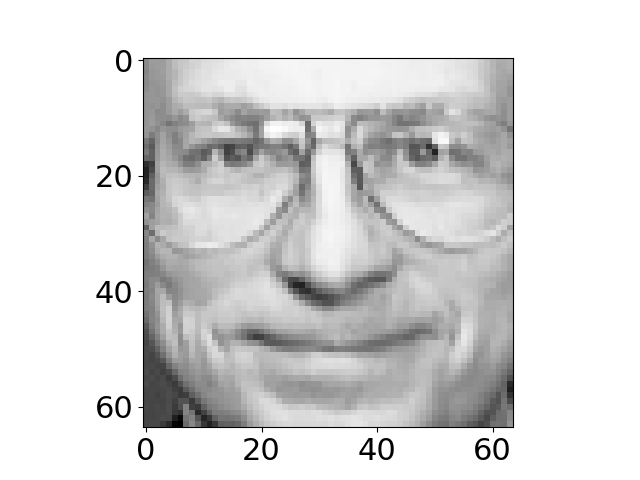
Figure: Data set from Olivetti Research Laboratory of faces.

Note that to display the face we had to reshape the appropriate row of the data matrix. This is because the images are turned into vectors by stacking columns of the image on top of each other to form a vector. The operation

im = np.reshape(Y[1, :].flatten(), (64, 64)).T}

recovers the original image into a matrix im by using the np.reshape function to return the vector to a matrix.

Visualizing the Eigenvectors

Each retained eigenvector is stored in the \(j\)th column of \(\mathbf{U}\). Each of these eigenvectors is associated with particular directions of variation in the original data. Principal component analysis implies that we can reconstruct any face by using a weighted sum of these eigenvectors where the weights for each face are given by the relevant vector of the latent variables, \(\mathbf{ z}_{i, :}\) and the diagonal elements of the matrix \(\mathbf{L}\). We can visualize the eigenvectors \(\mathbf{U}\) as images by performing the same reshape operation we used to recover the image associated with a data point above. Below we do this for the first nine eigenvectors of the Olivetti Faces data.

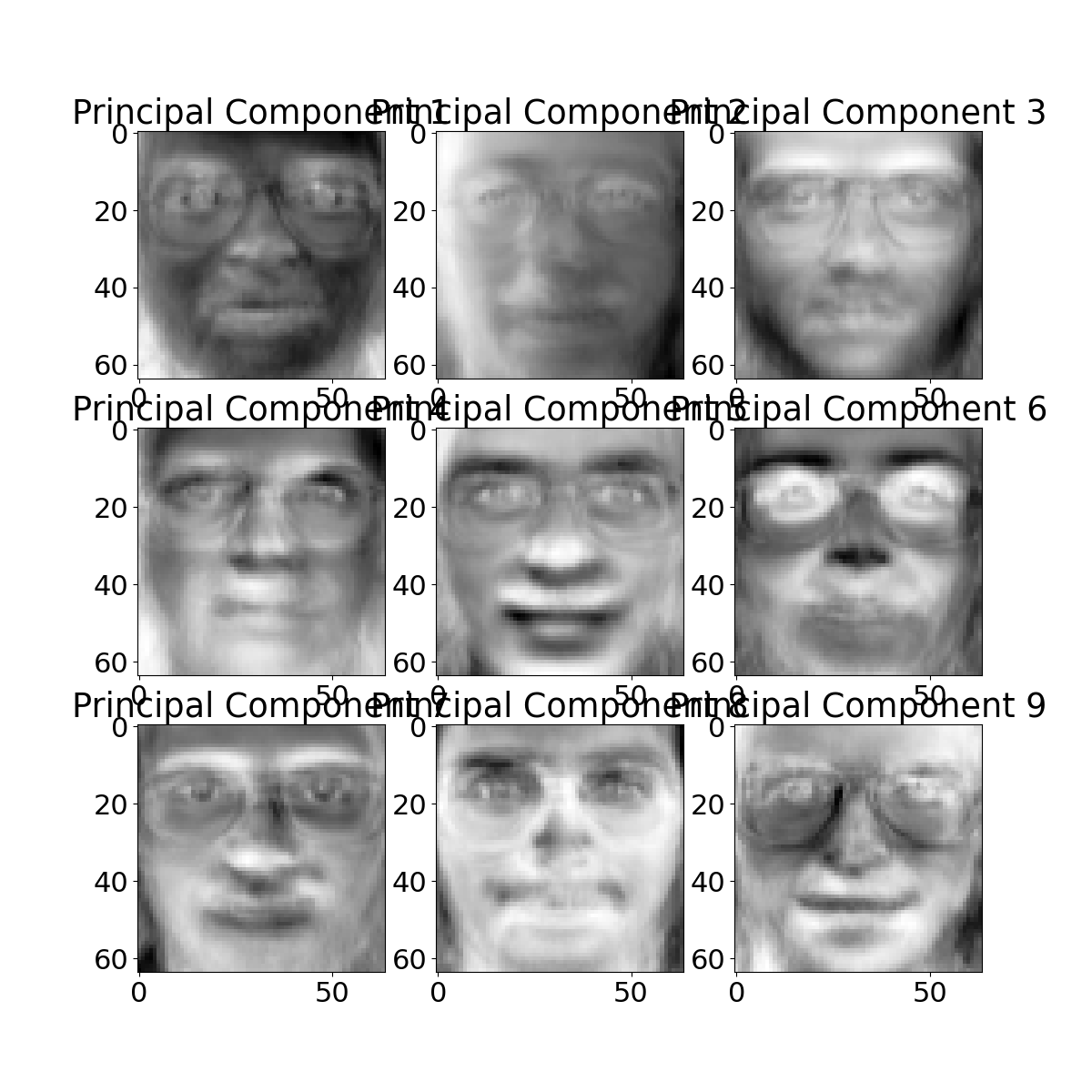
Figure: First 9 eigenvectors of the Olivetti faces data.

Reconstruction

We can now attempt to reconstruct a given training point from these eigenvectors. As we mentioned above, the reconstruction is dependent on the value of the latent variable and the weights from the matrix \(\mathbf{L}\). First let’s compute the value of the latent variables for the point we want to construct. Then we’ll use them to compute the weightings of each of the eigenvectors.

mu_x, C_x = posterior(Y, U, ell, sigma2)
reconstruction_weights = mu_x[display_index, :]*ell
print(reconstruction_weights)

This vector of reconstruction weights is applied to the ‘template images’ given by the eigenvectors to give us our reconstruction. Below we weight these templates and combine to form the reconstructed image, and show the comparison to the original image.

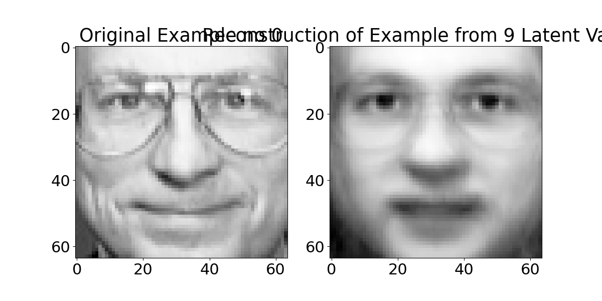
Figure: Reconstruction from the latent space of the faces data.

The quality of the reconstruction is a bit blurry, it can be improved by increasing the number of template images used (i.e. increasing the latent dimensionality).

Gene Expression

Each of the cells in your body stores your entire genetic code in your DNA, but at any one moment it is only ‘expressing’ a small portion of that code. Your cells are mainly constructed of protein, and these proteins are manufactured by first transcribing the DNA to RNA and then translating the RNA to protein. If the DNA is the cells hard drive, then one role of the RNA is to act like a cache of data that is being read from the hard drive at any one time. Gene expression arrays allow us to measure the quantity of different types of RNA in the cell, effectively analyzing what’s in the cache (although we have to destroy the cell or the tissue to access it). A gene expression experiment often consists of a time course or a series of experiments that characterise the gene expression of cells at any given time.

We will now load in one of the earliest gene expression data sets from a 1998 paper by Spellman et al., it consists of gene expression measurements of over six thousand genes in a range of conditions for brewer’s yeast. The experiment was designed for understanding the cell cycle of the genes. The expectation is that there should be oscillating signals inside the cell.

First we extract the principal components of the gene expression.

import pods

# load in data and replace missing values with zero
data=pods.datasets.spellman_yeast_cdc15()
Y = data['Y'].fillna(0)
q = 5
U, ell, sigma2 = ppca(Y, q)
mu_x, C_x = posterior(Y, U, ell, sigma2)

Now, looking through, we find that there is indeed a latent variable that appears to oscilate at approximately the right frequency. The 4th latent dimension (index=3) can be plotted across the time course as follows.

To reveal an oscillating shape. We can see which genes correspond to this shape by examining the associated column of \(\mathbf{U}\). Let’s augment our data matrix with this score.

gene_list = Y.T
gene_list['oscilation'] = np.sqrt(U[:, 3]**2)
gene_list.sort(columns='oscilation', ascending=False).index[:4]

We can look up the first three genes in this list which now ranks the genes according to how strongly they respond to the fourth latent dimension. The NCBI gene database allows us to search for the function of these genes. Looking at the function of the four genes that respond most strongly to the third latent variable they are all genes that encode histone proteins. The histone is thesupport scaffold for the DNA that ensures it folds correctly within the cell creating the nucleosomes. It seems to make sense that production of histone proteins should be strongly correlated with the cell cycle, as when the cell divides it needs to create a large number of histone proteins for creating the duplicated nucleosomes. The relevant links giving the descriptions of each gene given here: YDR224C, YDR225W, YBL003C and YNL030W.

When Dimensionality Reduction Fails

While dimensionality reduction is powerful, it’s important to understand when it can fail:

1. When the data really is high dimensional with no simpler structure
2. When the relationship between dimensions is highly nonlinear
3. When different parts of the data have different intrinsic dimensionality

import numpy as np
import matplotlib.pyplot as plt
import mlai.plot as plot
import mlai

The Swiss Roll Example

# Generate data that lies on a Swiss roll manifold
def generate_swiss_roll(n_points=1000):
    t = 1.5 * np.pi * (1 + 2 * np.random.rand(n_points))
    y = 21 * np.random.rand(n_points)
    x = t * np.cos(t)
    z = t * np.sin(t)
    return np.column_stack((x, y, z)), t

X, t = generate_swiss_roll()

fig = plt.figure(figsize=plot.big_wide_figsize)
ax = fig.add_subplot(111, projection='3d')
scatter = ax.scatter(X[:, 0], X[:, 1], X[:, 2], c=t, cmap='viridis')
ax.set_xlabel('$x$')
ax.set_ylabel('$y$') 
ax.set_zlabel('$z$')
plt.colorbar(scatter)

mlai.write_figure('swiss-roll.svg', directory='./dimred')

Figure: The Swiss roll dataset is a classic example of data with nonlinear structure. The color represents the position along the roll, showing how points that are far apart in the original space are actually close in the intrinsic manifold.

Common Failure Modes

This example shows data lying on a Swiss roll manifold. Linear dimensionality reduction methods like PCA will fail to capture the structure of this data, while nonlinear methods like t-SNE or UMAP may perform better.

Common failure modes include: 1. Using linear methods on nonlinear manifolds 2. Assuming global structure when only local structure exists 3. Not accounting for noise in the data

Visualization and Human Perception

The human visual system is remarkable - it represents our highest bandwidth connection to the world around us, with the optic tract carrying around 8.75 million bits per second of information to our brain (Koch et al., 2006). The “nerve” is misnamed, it is actually an extension of brain tissue, highlighting how central vision is to our cognitive architecture. Our (bidrectional) verbal communication is limited to around 2,000 bits per minute, but our eyes actively grab at information from our environment at vastly higher rates. This “active sensing” approach, see e.g. MacKay (1991) and O’Regan (2011), means we don’t passively receive visual information but actively construct our understanding through rapid eye movements called saccades that sample our environment hundreds of times per second.

Behind the Eye

Figure: Behind the Eye (MacKay, 1991) summarises MacKay’s Gifford Lectures, where MacKay uses the operation of the eye as a window on the operation of the brain.

The high-bandwidth visual channel makes visualization a powerful tool for communication and understanding. But it also makes us vulnerable to manipulation through misleading. Just as social media algorithms can manipulate our behavior through careful curation of information, indeed they sometimes manipulate us through our visual system, poorly designed or deliberately deceptive visualizations can lead us to incorrect conclusions by hijacking our natural visual processing capabilities.

Figure: Kevin O’Regan’s book, “Why Red Doesn’t Sound Like a Bell” is about the sensiorimotor perspective on feel and ranges from our senses to our consciousness.

The book, “Why Red Doesn’t Sound Like a Bell” by J. Kevin O’Regan (O’Regan, 2011) suggests a sensorimotor approach to understanding our consciousness. One that depends on how our senses interact with the world around us. The implication is that our consciousness is as much a function of our environment as of our mind. This is particularly interesting for social interaction, where our external environment is populated by other intelligent entities. If we accept this interpretation it would imply that we should pay a lot of attention to modes of human to human interaction when developing environments in which we can feel comfortable and able to perform.

In this lecture we’ll introduce the basics of visualisation through the lens of dimensionality reduction - techniques that help us represent high-dimensional data.

See Lawrence (2024) bandwidth, communication p. 10-12,16,21,29,31,34,38,41,44,65-67,76,81,90-91,104,115,149,196,214,216,235,237-238,302,334. See Lawrence (2024) MacKay, Donald p. 227-228,230-237,267-270. See Lawrence (2024) optic nerve/tract p. 205,235. See Lawrence (2024) O’Regan, Kevin p. 236-240,250,259,262-263,297,299. See Lawrence (2024) saccade p. 236,238,259-260,297,301. See Lawrence (2024) visual system/visual cortex p. 204-206,209,235-239,249-250,255,259,260,268-270,281,294,297,301,324,330.

Thanks!

For more information on these subjects and more you might want to check the following resources.

• company: Trent AI
• book: The Atomic Human
• twitter: @lawrennd
• podcast: The Talking Machines
• newspaper: Guardian Profile Page
• blog: http://inverseprobability.com

References