Latent Variables and Visualisation

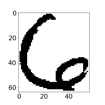
High Dimensional Data

• USPS Data Set Handwritten Digit
• 3648 dimensions (64 rows, 57 columns)
• Space contains much more than just this digit.

USPS Samples

Six Samples ❮ ❯

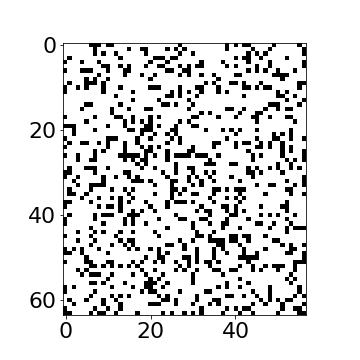
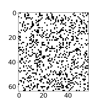
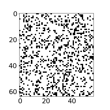
Simple Model of Digit

Probability of Random Image Generation

• Independent pixel model
  • Each pixel modeled as independent binomial trial
  • Probability of pixel being “on”\[\pi= \frac{849}{3,648} \approx 0.233\]
• Probability of original image \[p(\text{original six}) = \pi^{849}(1-\pi)^{2799} = 2.67 \times 10^{-860} \]

Probability of Random Image Generation

• This is astronomically small!
• Even sampling every nanosecond until end of universe won’t find it

Rotate a Prototype

PCA of Rotated Sixes

Interpoint Distances for Rotated Sixes

Low Dimensional Manifolds

• Pure rotation is too simple
  • In practice data may undergo several distortions.
• For high dimensional data with structure:
  • We expect fewer distortions than dimensions;
  • Therefore we expect the data to live on a lower dimensional manifold.
  • Conclusion: Deal with high dimensional data by looking for a lower dimensional non-linear embedding.

Latent Variables

• Hidden/unobservable variables we infer from observations
• Compression of complex data into simpler concepts
• Examples: motives, intentions, underlying causes

Robotics and State Estimation

• Robot state: position, speed, direction (latent)
• Sensors: only provide partial observations
• Uncertainty: true state must be inferred

Experimental Design and Confounders

• Confounders: hidden variables affecting outcomes
• Randomisation: breaks correlation with treatment
• Example: sunlight vs fertiliser effect

Probabilistic Framework

• Epistemic uncertainty: degree of belief as probability
• State space models: probabilistic graphical models
• This session: linear latent variable models

Your Personality

• High-dimensional questionnaire responses
• Few underlying traits drive behaviour
• Compression: many questions → few factors

Factor Analysis Model

\[ \mathbf{ y}= \mathbf{f}(\mathbf{ z}) + \boldsymbol{ \epsilon}, \]

\[ \mathbf{f}(\mathbf{ z}) = \mathbf{W}\mathbf{ z} \]

Closely Related to Linear Regression

\[ \mathbf{f}(\mathbf{ z}) = \begin{bmatrix} f_1(\mathbf{ z}) \\ f_2(\mathbf{ z}) \\ \vdots \\ f_p(\mathbf{ z})\end{bmatrix} \]

\[ f_j(\mathbf{ z}) = \mathbf{ w}_{j, :}^\top \mathbf{ z}, \]

\[ \epsilon_j \sim \mathscr{N}\left(0,\sigma^2_j\right). \]

Data Representation

\[ \mathbf{Y} = \begin{bmatrix} \mathbf{ y}_{1, :}^\top \\ \mathbf{ y}_{2, :}^\top \\ \vdots \\ \mathbf{ y}_{n, :}^\top\end{bmatrix}, \]

\[ \mathbf{F} = \mathbf{Z}\mathbf{W}^\top, \]

Latent Variables vs Linear Regression

Latent vs Observed Variables

• Regression: covariates \(\mathbf{Z}\) are observed
• Factor analysis: \(\mathbf{Z}\) are latent/unknown
• Solution: treat as probability distributions

\[ x_{i,j} \sim \mathscr{N}\left(0,1\right), \] and we can write the density governing the latent variable associated with a single point as, \[ \mathbf{ z}_{i, :} \sim \mathscr{N}\left(\mathbf{0},\mathbf{I}\right). \]

\[ \mathbf{f}_{i, :} = \mathbf{f}(\mathbf{ z}_{i, :}) = \mathbf{W}\mathbf{ z}_{i, :} \]

\[ \mathbf{f}_{i, :} \sim \mathscr{N}\left(\mathbf{0},\mathbf{W}\mathbf{W}^\top\right) \]

Data Distribution

\[ \mathbf{ y}_{i, :} = \sim \mathscr{N}\left(\mathbf{0},\mathbf{W}\mathbf{W}^\top + \boldsymbol{\Sigma}\right) \]

\[ \boldsymbol{\Sigma} = \begin{bmatrix}\sigma^2_{1} & 0 & 0 & 0\\ 0 & \sigma^2_{2} & 0 & 0\\ 0 & 0 & \ddots & 0\\ 0 & 0 & 0 & \sigma^2_p\end{bmatrix}. \]

Mean Vector

\[ \mathbf{ y}_{i, :} = \mathbf{W}\mathbf{ z}_{i, :} + \boldsymbol{ \mu}+ \boldsymbol{ \epsilon}_{i, :} \]

\[ \boldsymbol{ \mu}= \frac{1}{n} \sum_{i=1}^n \mathbf{ y}_{i, :}, \] \(\mathbf{C}= \mathbf{W}\mathbf{W}^\top + \boldsymbol{\Sigma}\)

Principal Component Analysis

Hotelling’s PCA (1933)

• Mathematical foundation for factor analysis
• Noiseless limit: \(\sigma^2_i \rightarrow 0\)
• Eigenvalue decomposition of covariance matrix

Hotelling (1933) took \(\sigma^2_i \rightarrow 0\) so \[ \mathbf{ y}_{i, :} \sim \lim_{\sigma^2 \rightarrow 0} \mathscr{N}\left(\mathbf{0},\mathbf{W}\mathbf{W}^\top + \sigma^2 \mathbf{I}\right). \]

Degenerate Covariance

\[ p(\mathbf{ y}_{i, :}|\mathbf{W}) = \lim_{\sigma^2 \rightarrow 0} \frac{1}{(2\pi)^\frac{p}{2} |\mathbf{W}\mathbf{W}^\top + \sigma^2 \mathbf{I}|^{\frac{1}{2}}} \exp\left(-\frac{1}{2}\mathbf{ y}_{i, :}\left[\mathbf{W}\mathbf{W}^\top+ \sigma^2 \mathbf{I}\right]^{-1}\mathbf{ y}_{i, :}\right), \]

Computation of the Marginal Likelihood

\[ \mathbf{ y}_{i,:}=\mathbf{W}\mathbf{ z}_{i,:}+\boldsymbol{ \epsilon}_{i,:},\quad \mathbf{ z}_{i,:} \sim \mathscr{N}\left(\mathbf{0},\mathbf{I}\right), \quad \boldsymbol{ \epsilon}_{i,:} \sim \mathscr{N}\left(\mathbf{0},\sigma^{2}\mathbf{I}\right) \]

\[ \mathbf{W}\mathbf{ z}_{i,:} \sim \mathscr{N}\left(\mathbf{0},\mathbf{W}\mathbf{W}^\top\right) \]

\[ \mathbf{W}\mathbf{ z}_{i, :} + \boldsymbol{ \epsilon}_{i, :} \sim \mathscr{N}\left(\mathbf{0},\mathbf{W}\mathbf{W}^\top + \sigma^2 \mathbf{I}\right) \]

Linear Latent Variable Model II

Probabilistic PCA Max. Likelihood Soln (Tipping and Bishop (1999))

\[p\left(\mathbf{Y}|\mathbf{W}\right)=\prod_{i=1}^{n}\mathscr{N}\left(\mathbf{ y}_{i, :}|\mathbf{0},\mathbf{W}\mathbf{W}^{\top}+\sigma^{2}\mathbf{I}\right)\]

Linear Latent Variable Model II

Probabilistic PCA Max. Likelihood Soln (Tipping and Bishop (1999)) \[ p\left(\mathbf{Y}|\mathbf{W}\right)=\prod_{i=1}^{n}\mathscr{N}\left(\mathbf{ y}_{i,:}|\mathbf{0},\mathbf{C}\right),\quad \mathbf{C}=\mathbf{W}\mathbf{W}^{\top}+\sigma^{2}\mathbf{I} \] \[ \log p\left(\mathbf{Y}|\mathbf{W}\right)=-\frac{n}{2}\log\left|\mathbf{C}\right|-\frac{1}{2}\text{tr}\left(\mathbf{C}^{-1}\mathbf{Y}^{\top}\mathbf{Y}\right)+\text{const.} \] If \(\mathbf{U}_{q}\) are first \(q\) principal eigenvectors of \(n^{-1}\mathbf{Y}^{\top}\mathbf{Y}\) and the corresponding eigenvalues are \(\boldsymbol{\Lambda}_{q}\), \[ \mathbf{W}=\mathbf{U}_{q}\mathbf{L}\mathbf{R}^{\top},\quad\mathbf{L}=\left(\boldsymbol{\Lambda}_{q}-\sigma^{2}\mathbf{I}\right)^{\frac{1}{2}} \] where \(\mathbf{R}\) is an arbitrary rotation matrix.

Probabilistic PCA

• Represent data, \(\mathbf{Y}\), with a lower dimensional set of latent variables \(\mathbf{Z}\).
• Assume a linear relationship of the form \[ \mathbf{ y}_{i,:}=\mathbf{W}\mathbf{ z}_{i,:}+\boldsymbol{ \epsilon}_{i,:}, \] where \[ \boldsymbol{ \epsilon}_{i,:} \sim \mathscr{N}\left(\mathbf{0},\sigma^2\mathbf{I}\right) \]

Probabilistic PCA

• PPCA defines a probabilistic model where:
  • Data is generated from latent variables through linear transformation
  • Gaussian noise is added to the transformed variables
  • Latent variables have standard Gaussian prior
• Maximum likelihood recovers classical PCA

Graphical model representing probabilistic PCA

Posterior for Principal Component Analysis

\[ p(\mathbf{ z}_{i, :} | \mathbf{ y}_{i, :}) \]

\[ p(\mathbf{ z}_{i, :} | \mathbf{ y}_{i, :}) \propto p(\mathbf{ y}_{i, :}|\mathbf{W}, \mathbf{ z}_{i, :}, \sigma^2) p(\mathbf{ z}_{i, :}) \]

\[ \log p(\mathbf{ z}_{i, :} | \mathbf{ y}_{i, :}) = \log p(\mathbf{ y}_{i, :}|\mathbf{W}, \mathbf{ z}_{i, :}, \sigma^2) + \log p(\mathbf{ z}_{i, :}) + \text{const} \]

\[ \log p(\mathbf{ z}_{i, :} | \mathbf{ y}_{i, :}) = -\frac{1}{2\sigma^2} (\mathbf{ y}_{i, :} - \mathbf{W}\mathbf{ z}_{i, :})^\top(\mathbf{ y}_{i, :} - \mathbf{W}\mathbf{ z}_{i, :}) - \frac{1}{2} \mathbf{ z}_{i, :}^\top \mathbf{ z}_{i, :} + \text{const} \]

Scikit-learn implementation PCA

Oil Flow Data

The Probabilistic PCA Model

Examples: Motion Capture Data

OSU Motion Capture Data: Run 1

Robot Navigation Example

• Example involving 215 observations of 30 access points.
• Infer location of ‘robot’ and access points.
• This is known as SLAM (simulataneous localization and mapping).

Interpretations of Principal Component Analysis

Principal Component Analysis

• PCA (Hotelling (1933)) is a linear embedding
• Today its presented as:
  • Rotate to find ‘directions’ in data with maximal variance
  • How do we find these directions?

\[ \mathbf{S}=\frac{1}{n}\sum_{i=1}^n\left(\mathbf{ y}_{i, :}-\boldsymbol{ \mu}\right)\left(\mathbf{ y}_{i, :} - \boldsymbol{ \mu}\right)^\top \]

Principal Component Analysis

• Find directions in the data, \(\mathbf{ z}= \mathbf{U}\mathbf{ y}\), for which variance is maximized.

Lagrangian

• Solution is found via constrained optimisation (which uses Lagrange multipliers): \[ L\left(\mathbf{u}_{1},\lambda_{1}\right)=\mathbf{u}_{1}^{\top}\mathbf{S}\mathbf{u}_{1}+\lambda_{1}\left(1-\mathbf{u}_{1}^{\top}\mathbf{u}_{1}\right) \]

• Gradient with respect to \(\mathbf{u}_{1}\) \[\frac{\text{d}L\left(\mathbf{u}_{1},\lambda_{1}\right)}{\text{d}\mathbf{u}_{1}}=2\mathbf{S}\mathbf{u}_{1}-2\lambda_{1}\mathbf{u}_{1}\]

Lagrangian

• Rearrange to form \[\mathbf{S}\mathbf{u}_{1}=\lambda_{1}\mathbf{u}_{1}.\] Which is known as an eigenvalue problem.
• Further directions that are orthogonal to the first can also be shown to be eigenvectors of the covariance.

PCA directions

Maximum variance directions are eigenvectors of the covariance matrix

Relationship to Matrix Factorization

• PCA is closely related to matrix factorisation.

• Instead of \(\mathbf{Z}\), \(\mathbf{W}\)

• Define Users \(\mathbf{U}\) and items \(\mathbf{V}\)

• Matrix factorisation: \[ f_{i, j} = \mathbf{u}_{i, :}^\top \mathbf{v}_{j, :} \] PCA: \[ f_{i, j} = \mathbf{ z}_{i, :}^\top \mathbf{ w}_{j, :} \]

PCA: Separating Model and Algorithm

• PCA introduced as latent variable model (a model).
• Solution is through an eigenvalue problem (an algorithm).
• This causes some confusion about what PCA is.

\[ \mathbf{Y}= \mathbf{V} \boldsymbol{\Lambda} \mathbf{U}^\top \]

\[ \mathbf{Y}^\top\mathbf{Y}= \mathbf{U}\boldsymbol{\Lambda}\mathbf{V}^\top\mathbf{V} \boldsymbol{\Lambda} \mathbf{U}^\top = \mathbf{U}\boldsymbol{\Lambda}^2 \mathbf{U}^\top \]

Separating Model and Algorithm

• Separation between model and algorithm is helpful conceptually.
• Even if in practice they conflate (e.g. deep neural networks).
• Sometimes difficult to pull apart.
• Helpful to revisit algorithms with modelling perspective in mind.
  • Probabilistic numerics

PCA Effectiveness

• So effective that used under different guises.
  • Latent semantic indexing
  • Eigenfaces (eigenvoices, eigengenes)
  • Phenomena of renaming common also in ML

Applying PCA

• If you have multivariate data.
  • Consider PCA as a first step.

Have you done PCA yet?

“Have you done PCA yet?” is data scientists equivalent of “Have you switched it off and on again yet?”

Derivation of PPCA

PPCA Marginal Likelihood

• Posterior density over latent variables given data and parameters
• Similar form to Bayesian regression posterior
• Key differences from Bayesian multiple output regression:
  • Independence across features vs data points
  • Different covariance structure

Computation of the Log Likelihood

• Model quality assessed using log likelihood
• Gaussian form allows efficient computation
• Key challenge: Inverting \(d\times d\) covariance matrix
• Solution: Exploit low-rank structure of \(\mathbf{W}\mathbf{W}^\top\)

Efficient Computation Strategy

• Low-rank structure \[\mathbf{C}= \mathbf{W}\mathbf{W}^\top + \sigma^2 \mathbf{I}\]
• SVD decomposition \[\mathbf{W}= \mathbf{U}\mathbf{L}\mathbf{R}^\top\]
• Optimisations
  • Determinant computation using eigenvalues
  • Woodbury matrix identity for inversion

Determinant Computation

• Efficient determinant \[\log |\mathbf{C}| = \sum_{i=1}^q\log (\ell_i^2 + \sigma^2) + (d-q)\log \sigma^2\]
• Only need \(q\) eigenvalues instead of \(d\)
• Computational complexity: \(O(q)\) vs \(O(d)\)

Woodbury Matrix Identity

• Inversion formula: \[(\sigma^2 \mathbf{I}+ \mathbf{W}\mathbf{W}^\top)^{-1} = \sigma^{-2}\mathbf{I}- \sigma^{-4}\mathbf{W}\mathbf{C}_x^{-1}\mathbf{W}^\top\]
• Invert \(q\times q\) matrix instead of \(d\times d\)
• Computational savings: \(O(q^3)\) vs \(O(d^3)\)
• Connection: \(\mathbf{C}_x\) is the posterior covariance from the latent space

Final Log Likelihood Formula

• Complete formula \[\log p(\mathbf{Y}|\mathbf{W}) = -\frac{n}{2} \sum_{i=1}^q\log (\ell_i^2 + \sigma^2) - \frac{n(d-q)}{2}\log \sigma^2 - \frac{\sigma^{-2}}{2} \text{tr}\left(\mathbf{Y}^\top \mathbf{Y}\right) + \frac{\sigma^{-4}}{2} \text{tr}\left(\mathbf{B}\mathbf{C}_x\mathbf{B}^\top\right)\]
• Key terms
  • Determinant: \(O(q)\) computation
  • Trace terms: \(O(nd)\) computation
  • Matrix inversions: \(O(q^3)\) instead of \(O(d^3)\)

Computational Efficiency

• Hadamard product: \(\text{tr}\left(\mathbf{Y}^\top\mathbf{Y}\right) = \sum_{i,j} (\mathbf{Y}\circ \mathbf{Y})_{i,j}\)
• Do (Y*Y).sum() not np.trace(Y.T@Y)
• Element-wise operations faster than matrix multiplication
• Overall complexity: \(O(nd+ q^3)\) vs \(O(d^3)\)
• Scales well for high-dimensional data with low latent dimension

Reconstruction of the Data

Given any posterior projection of a data point, we can replot the original data as a function of the input space.

We will now try to reconstruct the motion capture figure form some different places in the latent plot.

Other Data Sets to Explore

Below there are a few other data sets from pods you might want to explore with PCA. Both of them have \(p\)>\(n\) so you need to consider how to do the larger eigenvalue probleme efficiently without large demands on computer memory.

The data is actually quite high dimensional, and solving the eigenvalue problem in the high dimensional space can take some time. At this point we turn to a neat trick, you don’t have to solve the full eigenvalue problem in the \(d\times d\) covariance, you can choose instead to solve the related eigenvalue problem in the \(n\times n\) space, and in this case \(n=200\) which is much smaller than \(d\).

The original eigenvalue problem has the form \[ \mathbf{Y}^\top\mathbf{Y}\mathbf{U} = \mathbf{U}\boldsymbol{\Lambda} \] But if we premultiply by \(\mathbf{Y}\) then we can solve, \[ \mathbf{Y}\mathbf{Y}^\top\mathbf{Y}\mathbf{U} = \mathbf{Y}\mathbf{U}\boldsymbol{\Lambda} \] but it turns out that we can write \[ \mathbf{U}^\prime = \mathbf{Y}\mathbf{U} \Lambda^{\frac{1}{2}} \] where \(\mathbf{U}^\prime\) is an orthorormal matrix because \[ \left.\mathbf{U}^\prime\right.^\top\mathbf{U}^\prime = \Lambda^{-\frac{1}{2}}\mathbf{U}\mathbf{Y}^\top\mathbf{Y}\mathbf{U} \Lambda^{-\frac{1}{2}} \] and since \(\mathbf{U}\) diagonalises \(\mathbf{Y}^\top\mathbf{Y}\), \[ \mathbf{U}\mathbf{Y}^\top\mathbf{Y}\mathbf{U} = \Lambda \] then \[ \left.\mathbf{U}^\prime\right.^\top\mathbf{U}^\prime = \mathbf{I} \]

Olivetti Faces

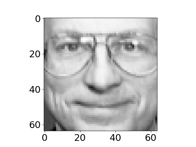
im = np.reshape(Y[1, :].flatten(), (64, 64)).T}

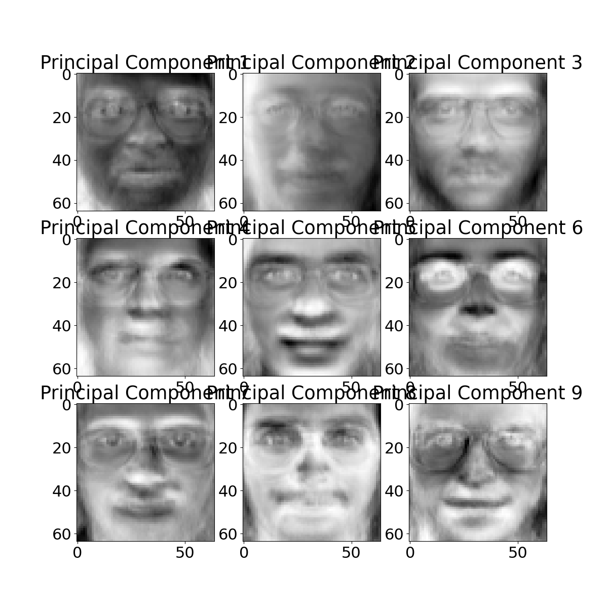
Visualizing the Eigenvectors

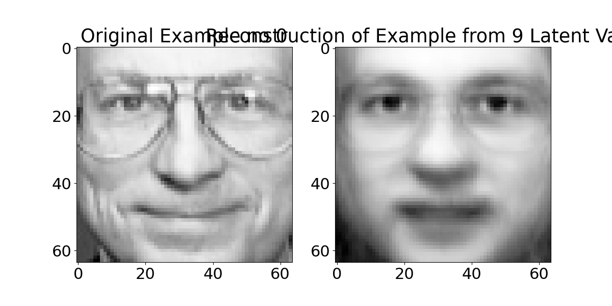
Reconstruction

Gene Expression

When Dimensionality Reduction Fails

• Dimensionality reduction can fail in several key scenarios:
  • Truly high dimensional data with no simpler structure
  • Highly nonlinear relationships between dimensions
  • Varying intrinsic dimensionality across data

The Swiss Roll Example

• Classic example of nonlinear structure
• 2D manifold embedded in 3D
• Linear methods like PCA fail
• Requires nonlinear methods (t-SNE, UMAP)

Common Failure Modes

• Key failure scenarios:
  • Linear methods on nonlinear manifolds
  • Assuming global structure when only local exists
  • Not accounting for noise

Visualization and Human Perception

• Human visual system is our highest bandwidth connection to the world
  • Optic tract: ~8.75 million bits/second
  • Verbal communication: only ~2,000 bits/minute
• Active sensing through rapid eye movements (saccades)
  • Not passive reception
  • Actively construct understanding
  • Hundreds of samples per second

Behind the Eye

Visualization and Human Perception

• Visualization is powerful for communication
• But can be vulnerable to manipulation
  • Similar to social media algorithms
  • Misleading visualizations can deceive
  • Can hijack natural visual processing