Week 3: Gaussian Processes II

[jupyter][google colab][reveal]

Neil D. Lawrence

Abstract: In this session we build on previous session to understand how to fit Gaussian processes and to look at how to build covariance functions.

ML Foundations Course Notebook Setup

We install some bespoke codes for creating and saving plots as well as loading data sets.

%%capture
%pip install notutils
%pip install pods
%pip install mlai

import notutils
import pods
import mlai
import mlai.plot as plot

%pip install gpy

Review

Marginal Likelihood

To understand the Gaussian process we’re going to build on our understanding of the marginal likelihood for Bayesian regression. In the session on we sampled directly from the weight vector, \(\mathbf{ w}\) and applied it to the basis matrix \(\boldsymbol{ \Phi}\) to obtain a sample from the prior and a sample from the posterior. It is often helpful to think of modeling techniques as generative models. To give some thought as to what the process for obtaining data from the model is. From the perspective of Gaussian processes, we want to start by thinking of basis function models, where the parameters are sampled from a prior, but move to thinking about sampling from the marginal likelihood directly.

Generating from the Model

A very important aspect of probabilistic modelling is to sample from your model to see what type of assumptions you are making about your data. In this case that involves a two stage process.

1. Sample a candiate parameter vector from the prior.
2. Place the candidate parameter vector in the likelihood and sample functions conditiond on that candidate vector.
3. Repeat to try and characterise the type of functions you are generating.

Given a prior variance (as defined above) we can now sample from the prior distribution and combine with a basis set to see what assumptions we are making about the functions a priori (i.e. before we’ve seen the data). Firstly we compute the basis function matrix. We will do it both for our training data, and for a range of prediction locations (x_pred).

Olympic Marathon Polynomial Sample

import numpy as np
import pods

data = pods.datasets.olympic_marathon_men()
x = data['X']
y = data['Y']

offset = y.mean()
scale = np.sqrt(y.var())
yhat = (y - offset)/scale
xlim = (1876,2044)

num_data = x.shape[0]

Now let’s build the basis matrices. We define the polynomial basis as follows.

from mlai import polynomial

import mlai

degree=4
alpha = 4
sigma2 = 0.1
num_pred_data = 100 # how many points to use for plotting predictions
x_pred = np.linspace(xlim[0], xlim[1], num_pred_data)[:, None] # input locations for predictions
data_limits=xlim
basis = mlai.Basis(polynomial, number=degree+1, data_limits=data_limits)
Phi_pred = basis.Phi(x_pred)
Phi = basis.Phi(x)

Sampling from the Prior

Now we will sample from the prior to produce a vector \(\mathbf{ w}\) and use it to plot a function which is representative of our belief before we fit the data. To do this we are going to use the properties of the Gaussian density and a sample from a standard normal using the function np.random.normal.

Let’s use this way of constructing samples from a Gaussian to check what functions look like a priori. The process will be as follows. First, we sample a random vector \(K\) dimensional from np.random.normal. Then we scale it by \(\sqrt{\alpha}\) to obtain a prior sample of \(\mathbf{ w}\).

K = degree + 1
z_vec = np.random.normal(size=K)
w_sample = z_vec*np.sqrt(alpha)
print(w_sample)

Now we can combine our sample from the prior with the basis functions to create a function,

import numpy as np

f_sample = Phi_pred@w_sample

Figure: Prior sample of \(\boldsymbol{ \Phi}\mathbf{ w}\) with \(\mathbf{ w}\) taken from the prior.

Note that we have carefully scaled our data using xlim to ensure that the polynomials don’t go too large. These samples should be well behaved.

Now we need to recompute the basis functions from above,

Mean Output

The prediction function can now be computed. In matrix form, the predictions can be computed as \[ \mathbf{ f}_s = \boldsymbol{ \Phi}\mathbf{ w}_s. \] This involves a matrix multiplication between a fixed matrix \(\boldsymbol{ \Phi}\) and a vector drawn from a distribution \(p(\mathbf{ w})\). Because \(\mathbf{ w}_s\) is drawn from a distribution, this imples that \(\mathbf{ f}_s\) should also be drawn from a distribution.

import numpy as np

f_sample = Phi_pred@w_sample

Now let’s loop through some samples and plot various functions as samples from this system,

Figure: Samples of \(\boldsymbol{ \Phi}\mathbf{ w}\) with \(\mathbf{ w}\) taken from the prior.

There are two distributions we are interested in though. We have just been sampling from the prior distribution to see what sort of functions we get before looking at the data. In Bayesian inference, we also need to compute the posterior distribution and sample from that density.

Function Space View

The process we have used to generate the samples is a two stage process. To obtain each function, we first generated a sample from the prior, \[ \mathbf{ w}\sim \mathscr{N}\left(\mathbf{0},\alpha \mathbf{I}\right) \] then if we compose our basis matrix, \(\boldsymbol{ \Phi}\) from the basis functions associated with each row then we get, \[ \boldsymbol{ \Phi}= \begin{bmatrix}\boldsymbol{ \phi}(\mathbf{ x}_1) \\ \vdots \\ \boldsymbol{ \phi}(\mathbf{ x}_n)\end{bmatrix} \] then we can write down the vector of function values, as evaluated at \[ \mathbf{ f}= \begin{bmatrix} f_1 \\ \vdots \\ f_n\end{bmatrix} \] in the form \[ \mathbf{ f}= \boldsymbol{ \Phi}\mathbf{ w}. \]

Now we can use standard properties of multivariate Gaussians to write down the probability density that is implied over \(\mathbf{ f}\). In particular we know that if \(\mathbf{ w}\) is sampled from a multivariate normal (or multivariate Gaussian) with covariance \(\alpha \mathbf{I}\) and zero mean, then assuming that \(\boldsymbol{ \Phi}\) is a deterministic matrix (i.e. it is not sampled from a probability density) then the vector \(\mathbf{ f}\) will also be distributed according to a zero mean multivariate normal as follows, \[ \mathbf{ f}\sim \mathscr{N}\left(\mathbf{0},\alpha \boldsymbol{ \Phi}\boldsymbol{ \Phi}^\top\right). \]

The question now is, what happens if we sample \(\mathbf{ f}\) directly from this density, rather than first sampling \(\mathbf{ w}\) and then multiplying by \(\boldsymbol{ \Phi}\). Let’s try this. First of all we define the covariance as \[ \mathbf{K}= \alpha \boldsymbol{ \Phi}\boldsymbol{ \Phi}^\top. \]

K = alpha*Phi_pred@Phi_pred.T

Now we can use the np.random.multivariate_normal command for sampling from a multivariate normal with covariance given by \(\mathbf{K}\) and zero mean,

fig, ax = plt.subplots(figsize=plot.big_wide_figsize)
for i in range(10):
    f_sample = np.random.multivariate_normal(mean=np.zeros(x_pred.size), cov=K)
    ax.plot(x_pred.flatten(), f_sample.flatten(), linewidth=2)
    
mlai.write_figure('gp-sample-basis-function.svg', directory='./kern')

Figure: Samples directly from the covariance function implied by the basis function based covariance, \(\alpha \boldsymbol{ \Phi}\boldsymbol{ \Phi}^\top\).

The samples appear very similar to those which we obtained indirectly. That is no surprise because they are effectively drawn from the same mutivariate normal density. However, when sampling \(\mathbf{ f}\) directly we created the covariance for \(\mathbf{ f}\). We can visualise the form of this covaraince in an image in python with a colorbar to show scale.

Figure: Covariance of the function implied by the basis set \(\alpha\boldsymbol{ \Phi}\boldsymbol{ \Phi}^\top\).

This image is the covariance expressed between different points on the function. In regression we normally also add independent Gaussian noise to obtain our observations \(\mathbf{ y}\), \[ \mathbf{ y}= \mathbf{ f}+ \boldsymbol{\epsilon} \] where the noise is sampled from an independent Gaussian distribution with variance \(\sigma^2\), \[ \epsilon \sim \mathscr{N}\left(\mathbf{0},\sigma^2\mathbf{I}\right). \] we can use properties of Gaussian variables, i.e. the fact that sum of two Gaussian variables is also Gaussian, and that it’s covariance is given by the sum of the two covariances, whilst the mean is given by the sum of the means, to write down the marginal likelihood, \[ \mathbf{ y}\sim \mathscr{N}\left(\mathbf{0},\boldsymbol{ \Phi}\boldsymbol{ \Phi}^\top +\sigma^2\mathbf{I}\right). \] Sampling directly from this density gives us the noise corrupted functions,

Figure: Samples directly from the covariance function implied by the noise corrupted basis function based covariance, \(\alpha \boldsymbol{ \Phi}\boldsymbol{ \Phi}^\top + \sigma^2 \mathbf{I}\).

where the effect of our noise term is to roughen the sampled functions, we can also increase the variance of the noise to see a different effect,

sigma2 = 1.
K = alpha*Phi_pred@Phi_pred.T + sigma2*np.eye(x_pred.size)

fig, ax = plt.subplots(figsize=plot.big_wide_figsize)
for i in range(10):
    y_sample = np.random.multivariate_normal(mean=np.zeros(x_pred.size), cov=K)
    plt.plot(x_pred.flatten(), y_sample.flatten())
    
mlai.write_figure('gp-sample-basis-function-plus-large-noise.svg', 
                  directory='./kern')

Figure: Samples directly from the covariance function implied by the noise corrupted basis function based covariance, \(\alpha \boldsymbol{ \Phi}\boldsymbol{ \Phi}^\top + \mathbf{I}\).

Non-degenerate Gaussian Processes

The process described above is degenerate. The covariance function is of rank at most \(h\) and since the theoretical amount of data could always increase \(n\rightarrow \infty\), the covariance function is not full rank. This means as we increase the amount of data to infinity, there will come a point where we can’t normalize the process because the multivariate Gaussian has the form, \[ \mathscr{N}\left(\mathbf{ f}|\mathbf{0},\mathbf{K}\right) = \frac{1}{\left(2\pi\right)^{\frac{n}{2}}\det{\mathbf{K}}^\frac{1}{2}} \exp\left(-\frac{\mathbf{ f}^\top\mathbf{K}\mathbf{ f}}{2}\right) \] and a non-degenerate kernel matrix leads to \(\det{\mathbf{K}} = 0\) defeating the normalization (it’s equivalent to finding a projection in the high dimensional Gaussian where the variance of the the resulting univariate Gaussian is zero, i.e. there is a null space on the covariance, or alternatively you can imagine there are one or more directions where the Gaussian has become the delta function).

In the machine learning field, it was Radford Neal (Neal, 1994) that realized the potential of the next step. In his 1994 thesis, he was considering Bayesian neural networks, of the type we described above, and in considered what would happen if you took the number of hidden nodes, or neurons, to infinity, i.e. \(h\rightarrow \infty\).

Figure: Page 37 of Radford Neal’s 1994 thesis

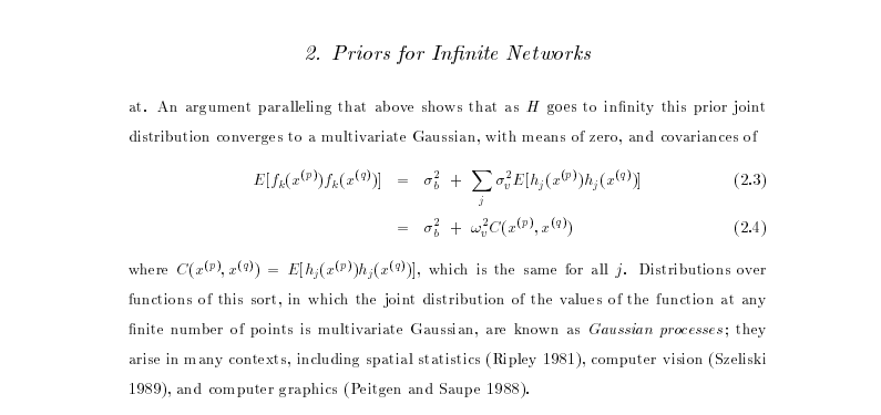
In loose terms, what Radford considers is what happens to the elements of the covariance function, \[ \begin{align*} k_f\left(\mathbf{ x}_i, \mathbf{ x}_j\right) & = \alpha \boldsymbol{ \phi}\left(\mathbf{W}_1, \mathbf{ x}_i\right)^\top \boldsymbol{ \phi}\left(\mathbf{W}_1, \mathbf{ x}_j\right)\\ & = \alpha \sum_k \phi\left(\mathbf{ w}^{(1)}_k, \mathbf{ x}_i\right) \phi\left(\mathbf{ w}^{(1)}_k, \mathbf{ x}_j\right) \end{align*} \] if instead of considering a finite number you sample infinitely many of these activation functions, sampling parameters from a prior density, \(p(\mathbf{ v})\), for each one,

\[ k_f\left(\mathbf{ x}_i, \mathbf{ x}_j\right) = \alpha \int \phi\left(\mathbf{ w}^{(1)}, \mathbf{ x}_i\right) \phi\left(\mathbf{ w}^{(1)}, \mathbf{ x}_j\right) p(\mathbf{ w}^{(1)}) \text{d}\mathbf{ w}^{(1)} \] And that’s not only for Gaussian \(p(\mathbf{ v})\). In fact this result holds for a range of activations, and a range of prior densities because of the central limit theorem.

To write it in the form of a probabilistic program, as long as the distribution for \(\phi_i\) implied by this short probabilistic program, \[ \begin{align*} \mathbf{ v}& \sim p(\cdot)\\ \phi_i & = \phi\left(\mathbf{ v}, \mathbf{ x}_i\right), \end{align*} \] has finite variance, then the result of taking the number of hidden units to infinity, with appropriate scaling, is also a Gaussian process.

Further Reading

To understand this argument in more detail, I highly recommend reading chapter 2 of Neal’s thesis (Neal, 1994), which remains easy to read and clear today. Indeed, for readers interested in Bayesian neural networks, both Raford Neal’s and David MacKay’s PhD thesis (MacKay, 1992) remain essential reading. Both theses embody a clarity of thought, and an ability to weave together threads from different fields that was the business of machine learning in the 1990s. Radford and David were also pioneers in making their software widely available and publishing material on the web.

Gaussian Process

In our we sampled from the prior over paraemters. Through the properties of multivariate Gaussian densities this prior over parameters implies a particular density for our data observations, \(\mathbf{ y}\). In this session we sampled directly from this distribution for our data, avoiding the intermediate weight-space representation. This is the approach taken by Gaussian processes. In a Gaussian process you specify the covariance function directly, rather than implicitly through a basis matrix and a prior over parameters. Gaussian processes have the advantage that they can be nonparametric, which in simple terms means that they can have infinite basis functions. In the lectures we introduced the exponentiated quadratic covariance, also known as the RBF or the Gaussian or the squared exponential covariance function. This covariance function is specified by \[ k(\mathbf{ x}, \mathbf{ x}^\prime) = \alpha \exp\left( -\frac{\left\Vert \mathbf{ x}-\mathbf{ x}^\prime\right\Vert^2}{2\ell^2}\right), \] where \(\left\Vert\mathbf{ x}- \mathbf{ x}^\prime\right\Vert^2\) is the squared distance between the two input vectors \[ \left\Vert\mathbf{ x}- \mathbf{ x}^\prime\right\Vert^2 = (\mathbf{ x}- \mathbf{ x}^\prime)^\top (\mathbf{ x}- \mathbf{ x}^\prime) \] Let’s build a covariance matrix based on this function. First we define the form of the covariance function,

from mlai import eq_cov

We can use this to compute directly the covariance for \(\mathbf{ f}\) at the points given by x_pred. Let’s define a new function K() which does this,

from mlai import Kernel

Now we can image the resulting covariance,

kernel = mlai.Kernel(function=mlai.eq_cov, variance=1., lengthscale=10.)
K = kernel.K(x_pred, x_pred)

To visualise the covariance between the points we can use the imshow function in matplotlib.

Finally, we can sample functions from the marginal likelihood.

Exercise 1

Moving Parameters Have a play with the parameters for this covariance function (the lengthscale and the variance) and see what effects the parameters have on the types of functions you observe.

Bayesian Inference by Rejection Sampling

One view of Bayesian inference is to assume we are given a mechanism for generating samples, where we assume that mechanism is representing an accurate view on the way we believe the world works.

This mechanism is known as our prior belief.

We combine our prior belief with our observations of the real world by discarding all those prior samples that are inconsistent with our observations. The likelihood defines mathematically what we mean by inconsistent with the observations. The higher the noise level in the likelihood, the looser the notion of consistent.

The samples that remain are samples from the posterior.

This approach to Bayesian inference is closely related to two sampling techniques known as rejection sampling and importance sampling. It is realized in practice in an approach known as approximate Bayesian computation (ABC) or likelihood-free inference.

In practice, the algorithm is often too slow to be practical, because most samples will be inconsistent with the observations and as a result the mechanism must be operated many times to obtain a few posterior samples.

However, in the Gaussian process case, when the likelihood also assumes Gaussian noise, we can operate this mechanism mathematically, and obtain the posterior density analytically. This is the benefit of Gaussian processes.

First, we will load in two python functions for computing the covariance function.

Next, we sample from a multivariate normal density (a multivariate Gaussian), using the covariance function as the covariance matrix.

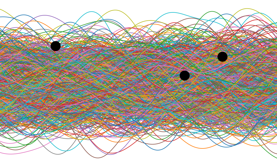
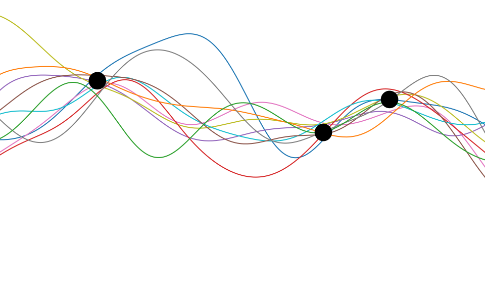
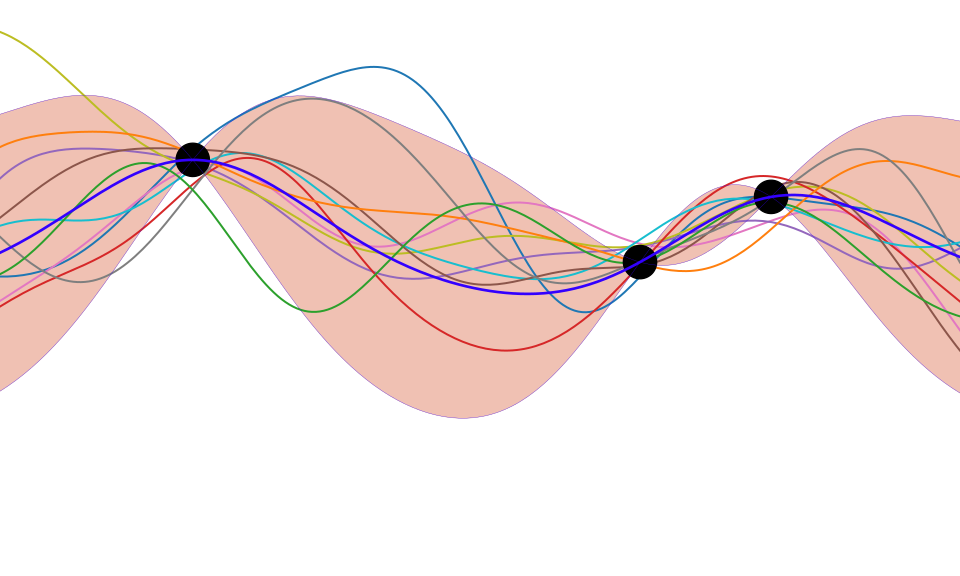
Figure: One view of Bayesian inference is we have a machine for generating samples (the prior), and we discard all samples inconsistent with our data, leaving the samples of interest (the posterior). This is a rejection sampling view of Bayesian inference. The Gaussian process allows us to do this analytically by multiplying the prior by the likelihood.

Making Predictions with Gaussian Process

The Gaussian process perspective takes the marginal likelihood of the data to be a joint Gaussian density with a covariance given by \(\mathbf{K}\). So the model likelihood is of the form, \[ p(\mathbf{ y}|\mathbf{X}) = \frac{1}{(2\pi)^{\frac{n}{2}}|\mathbf{K}|^{\frac{1}{2}}} \exp\left(-\frac{1}{2}\mathbf{ y}^\top \left(\mathbf{K}+\sigma^2 \mathbf{I}\right)^{-1}\mathbf{ y}\right) \] where the input data, \(\mathbf{X}\), influences the density through the covariance matrix, \(\mathbf{K}\) whose elements are computed through the covariance function, \(k(\mathbf{ x}, \mathbf{ x}^\prime)\).

This means that the negative log likelihood (the objective function) is given by, \[ E(\boldsymbol{\theta}) = \frac{1}{2} \log |\mathbf{K}| + \frac{1}{2} \mathbf{ y}^\top \left(\mathbf{K}+ \sigma^2\mathbf{I}\right)^{-1}\mathbf{ y} \] where the parameters of the model are also embedded in the covariance function, they include the parameters of the kernel (such as lengthscale and variance), and the noise variance, \(\sigma^2\). Let’s create a set of classes in python for storing these variables.

from mlai import ProbMapModel

from mlai import GP

Making Predictions

We now have a probability density that represents functions. How do we make predictions with this density? The density is known as a process because it is consistent. By consistency, here, we mean that the model makes predictions for \(\mathbf{ f}\) that are unaffected by future values of \(\mathbf{ f}^*\) that are currently unobserved (such as test points). If we think of \(\mathbf{ f}^*\) as test points, we can still write down a joint probability density over the training observations, \(\mathbf{ f}\) and the test observations, \(\mathbf{ f}^*\). This joint probability density will be Gaussian, with a covariance matrix given by our covariance function, \(k(\mathbf{ x}_i, \mathbf{ x}_j)\). \[ \begin{bmatrix}\mathbf{ f}\\ \mathbf{ f}^*\end{bmatrix} \sim \mathscr{N}\left(\mathbf{0},\begin{bmatrix} \mathbf{K}& \mathbf{K}_\ast \\ \mathbf{K}_\ast^\top & \mathbf{K}_{\ast,\ast}\end{bmatrix}\right) \] where here \(\mathbf{K}\) is the covariance computed between all the training points, \(\mathbf{K}_\ast\) is the covariance matrix computed between the training points and the test points and \(\mathbf{K}_{\ast,\ast}\) is the covariance matrix computed betwen all the tests points and themselves. To be clear, let’s compute these now for our example, using x and y for the training data (although y doesn’t enter the covariance) and x_pred as the test locations.

# set covariance function parameters
variance = 16.0
lengthscale = 8
# set noise variance
sigma2 = 0.05

kernel = Kernel(eq_cov, variance=variance, lengthscale=lengthscale)
K = kernel.K(x, x)
K_star = kernel.K(x, x_pred)
K_starstar = kernel.K(x_pred, x_pred)

Now we use this structure to visualise the covariance between test data and training data. This structure is how information is passed between test and training data. Unlike the maximum likelihood formalisms we’ve been considering so far, the structure expresses correlation between our different data points. However, just like the we now have a joint density between some variables of interest. In particular we have the joint density over \(p(\mathbf{ f}, \mathbf{ f}^*)\). The joint density is Gaussian and zero mean. It is specified entirely by the covariance matrix, \(\mathbf{K}\). That covariance matrix is, in turn, defined by a covariance function. Now we will visualise the form of that covariance in the form of the matrix, \[ \begin{bmatrix} \mathbf{K}& \mathbf{K}_\ast \\ \mathbf{K}_\ast^\top & \mathbf{K}_{\ast,\ast}\end{bmatrix} \]

Figure: Different blocks of the covariance function. The upper left block is the covariance of the training data with itself, \(\mathbf{K}\). The top right is the cross covariance between training data (rows) and prediction locations (columns). The lower left is the same matrix transposed. The bottom right is the covariance matrix of the test data with itself.

There are four blocks to this plot. The upper left block is the covariance of the training data with itself, \(\mathbf{K}\). We see some structure here due to the missing data from the first and second world wars. Alongside this covariance (to the right and below) we see the cross covariance between the training and the test data (\(\mathbf{K}_*\) and \(\mathbf{K}_*^\top\)). This is giving us the covariation between our training and our test data. Finally the lower right block The banded structure we now observe is because some of the training points are near to some of the test points. This is how we obtain ‘communication’ between our training data and our test data. If there is no structure in \(\mathbf{K}_*\) then our belief about the test data simply matches our prior.

The Importance of the Covariance Function

The covariance function encapsulates our assumptions about the data. The equations for the distribution of the prediction function, given the training observations, are highly sensitive to the covariation between the test locations and the training locations as expressed by the matrix \(\mathbf{K}_*\). We defined a matrix \(\mathbf{A}\) which allowed us to express our conditional mean in the form, \[ \boldsymbol{ \mu}_f= \mathbf{A}^\top \mathbf{ y}, \] where \(\mathbf{ y}\) were our training observations. In other words our mean predictions are always a linear weighted combination of our training data. The weights are given by computing the covariation between the training and the test data (\(\mathbf{K}_*\)) and scaling it by the inverse covariance of the training data observations, \(\left[\mathbf{K}+ \sigma^2 \mathbf{I}\right]^{-1}\). This inverse is the main computational object that needs to be resolved for a Gaussian process. It has a computational burden which is \(O(n^3)\) and a storage burden which is \(O(n^2)\). This makes working with Gaussian processes computationally intensive for the situation where \(n>10,000\).

Figure: Introduction to Gaussian processes given by Neil Lawrence at the 2014 Gaussian process Winter School at the University of Sheffield.

Parameter Optimisation

Improving the Numerics

In practice we shouldn’t be using matrix inverse directly to solve the GP system. One more stable way is to compute the Cholesky decomposition of the kernel matrix. The log determinant of the covariance can also be derived from the Cholesky decomposition.

import scipy.linalg as la

from mlai import update_inverse

# Bind the updated inverse to our GP model
GP.update_inverse = update_inverse

Capacity Control

Gaussian processes are sometimes seen as part of a wider family of methods known as kernel methods. Kernel methods are also based around covariance functions, but in the field they are known as Mercer kernels. Mercer kernels have interpretations as inner products in potentially infinite dimensional Hilbert spaces. This interpretation arises because, if we take \(\alpha=1\), then the kernel can be expressed as \[ \mathbf{K}= \boldsymbol{ \Phi}\boldsymbol{ \Phi}^\top \] which imples the elements of the kernel are given by, \[ k(\mathbf{ x}, \mathbf{ x}^\prime) = \boldsymbol{ \phi}(\mathbf{ x})^\top \boldsymbol{ \phi}(\mathbf{ x}^\prime). \] So we see that the kernel function is developed from an inner product between the basis functions. Mercer’s theorem tells us that any valid positive definite function can be expressed as this inner product but with the caveat that the inner product could be infinite length. This idea has been used quite widely to kernelize algorithms that depend on inner products. The kernel functions are equivalent to covariance functions and they are parameterized accordingly. In the kernel modeling community it is generally accepted that kernel parameter estimation is a difficult problem and the normal solution is to cross validate to obtain parameters. This can cause difficulties when a large number of kernel parameters need to be estimated. In Gaussian process modelling kernel parameter estimation (in the simplest case proceeds) by maximum likelihood. This involves taking gradients of the likelihood with respect to the parameters of the covariance function.

Gradients of the Likelihood

The easiest conceptual way to obtain the gradients is a two step process. The first step involves taking the gradient of the likelihood with respect to the covariance function, the second step involves considering the gradient of the covariance function with respect to its parameters.

Overall Process Scale

In general we won’t be able to find parameters of the covariance function through fixed point equations, we will need to do gradient based optimization.

Capacity Control and Data Fit

The objective function can be decomposed into two terms, a capacity control term, and a data fit term. The capacity control term is the log determinant of the covariance. The data fit term is the matrix inner product between the data and the inverse covariance.

Learning Covariance Parameters

Can we determine covariance parameters from the data?

\[ \mathscr{N}\left(\mathbf{ y}|\mathbf{0},\mathbf{K}\right)=\frac{1}{(2\pi)^\frac{n}{2}{\det{\mathbf{K}}^{\frac{1}{2}}}}{\exp\left(-\frac{\mathbf{ y}^{\top}\mathbf{K}^{-1}\mathbf{ y}}{2}\right)} \]

\[ \begin{aligned} \mathscr{N}\left(\mathbf{ y}|\mathbf{0},\mathbf{K}\right)=\frac{1}{(2\pi)^\frac{n}{2}\color{blue}{\det{\mathbf{K}}^{\frac{1}{2}}}}\color{red}{\exp\left(-\frac{\mathbf{ y}^{\top}\mathbf{K}^{-1}\mathbf{ y}}{2}\right)} \end{aligned} \]

\[ \begin{aligned} \log \mathscr{N}\left(\mathbf{ y}|\mathbf{0},\mathbf{K}\right)=&\color{blue}{-\frac{1}{2}\log\det{\mathbf{K}}}\color{red}{-\frac{\mathbf{ y}^{\top}\mathbf{K}^{-1}\mathbf{ y}}{2}} \\ &-\frac{n}{2}\log2\pi \end{aligned} \]

\[ E(\boldsymbol{ \theta}) = \color{blue}{\frac{1}{2}\log\det{\mathbf{K}}} + \color{red}{\frac{\mathbf{ y}^{\top}\mathbf{K}^{-1}\mathbf{ y}}{2}} \]

Capacity Control through the Determinant

The parameters are inside the covariance function (matrix). \[k_{i, j} = k(\mathbf{ x}_i, \mathbf{ x}_j; \boldsymbol{ \theta})\]

\[\mathbf{K}= \mathbf{R}\boldsymbol{ \Lambda}^2 \mathbf{R}^\top\]

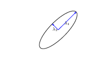
\(\boldsymbol{ \Lambda}\) represents distance on axes. \(\mathbf{R}\) gives rotation.

• \(\boldsymbol{ \Lambda}\) is diagonal, \(\mathbf{R}^\top\mathbf{R}= \mathbf{I}\).
• Useful representation since \(\det{\mathbf{K}} = \det{\boldsymbol{ \Lambda}^2} = \det{\boldsymbol{ \Lambda}}^2\).

Figure: The determinant of the covariance is dependent only on the eigenvalues. It represents the ‘footprint’ of the Gaussian.

Quadratic Data Fit

Figure: The data fit term of the Gaussian process is a quadratic loss centered around zero. This has eliptical contours, the principal axes of which are given by the covariance matrix.

Data Fit Term

x = np.linspace(-1, 1, 6)[:, np.newaxis]
xtest = np.linspace(x_lim[0], x_lim[1], 200)[:, np.newaxis]

# True data
true_kernel = Kernel(eq_cov, name='Exponentiated Quadratic', shortname='eq', lengthscale=1)
K = true_kernel.K(x) + np.eye(6)*0.01 
y = np.random.multivariate_normal(np.zeros((6,)), K, 1).T

# Fitted model
kernel = Kernel(eq_cov, name='Exponentiated Quadratic', shortname='eq', lengthscale=1)
gp = GP(x, y, sigma2=0.01, kernel=kernel)

Figure: Variation in the data fit term, the capacity term and the negative log likelihood for different lengthscales.

Exponentiated Quadratic Covariance

The exponentiated quadratic covariance, also known as the Gaussian covariance or the RBF covariance and the squared exponential. Covariance between two points is related to the negative exponential of the squared distnace between those points. This covariance function can be derived in a few different ways: as the infinite limit of a radial basis function neural network, as diffusion in the heat equation, as a Gaussian filter in Fourier space or as the composition as a series of linear filters applied to a base function.

The covariance takes the following form, \[ k(\mathbf{ x}, \mathbf{ x}^\prime) = \alpha \exp\left(-\frac{\left\Vert \mathbf{ x}-\mathbf{ x}^\prime \right\Vert_2^2}{2\ell^2}\right) \] where \(\ell\) is the length scale or time scale of the process and \(\alpha\) represents the overall process variance.

Figure: The exponentiated quadratic covariance function.

Olympic Marathon Data

Gold medal times for Olympic Marathon since 1896. Marathons before 1924 didn’t have a standardized distance. Present results using pace per km. In 1904 Marathon was badly organized leading to very slow times.

Image from Wikimedia Commons

The Olympic Marathon data is a standard dataset for regression modelling. The data consists of the pace of Olympic Gold Medal Marathon winners for the Olympics from 1896 to present. Let’s load in the data and plot.

%pip install pods

import numpy as np
import pods

data = pods.datasets.olympic_marathon_men()
x = data['X']
y = data['Y']

offset = y.mean()
scale = np.sqrt(y.var())
yhat = (y - offset)/scale

Figure: Olympic marathon pace times since 1896.

Things to notice about the data include the outlier in 1904, in that year the Olympics was in St Louis, USA. Organizational problems and challenges with dust kicked up by the cars following the race meant that participants got lost, and only very few participants completed. More recent years see more consistently quick marathons.

Gaussian Process Fit

Our first objective will be to perform a Gaussian process fit to the data, we’ll do this using the GPy software.

import GPy

m_full = GPy.models.GPRegression(x,yhat)
_ = m_full.optimize() # Optimize parameters of covariance function

The first command sets up the model, then m_full.optimize() optimizes the parameters of the covariance function and the noise level of the model. Once the fit is complete, we’ll try creating some test points, and computing the output of the GP model in terms of the mean and standard deviation of the posterior functions between 1870 and 2030. We plot the mean function and the standard deviation at 200 locations. We can obtain the predictions using y_mean, y_var = m_full.predict(xt)

xt = np.linspace(1870,2030,200)[:,np.newaxis]
yt_mean, yt_var = m_full.predict(xt)
yt_sd=np.sqrt(yt_var)

Now we plot the results using the helper function in mlai.plot.

Figure: Gaussian process fit to the Olympic Marathon data. The error bars are too large, perhaps due to the outlier from 1904.

Fit Quality

In the fit we see that the error bars (coming mainly from the noise variance) are quite large. This is likely due to the outlier point in 1904, ignoring that point we can see that a tighter fit is obtained. To see this make a version of the model, m_clean, where that point is removed.

x_clean=np.vstack((x[0:2, :], x[3:, :]))
y_clean=np.vstack((yhat[0:2, :], yhat[3:, :]))

m_clean = GPy.models.GPRegression(x_clean,y_clean)
_ = m_clean.optimize()

Figure: Gaussian process fit to the Olympic Marathon data. Here we’ve removed the outlier from 1904.

Gene Expression Example

We now consider an example in gene expression. Gene expression is the measurement of mRNA levels expressed in cells. These mRNA levels show which genes are ‘switched on’ and producing data. In the example we will use a Gaussian process to determine whether a given gene is active, or we are merely observing a noise response.

Della Gatta Gene Data

• Given given expression levels in the form of a time series from Della Gatta et al. (2008).

import numpy as np
import pods

data = pods.datasets.della_gatta_TRP63_gene_expression(data_set='della_gatta',gene_number=937)

x = data['X']
y = data['Y']

offset = y.mean()
scale = np.sqrt(y.var())

Figure: Gene expression levels over time for a gene from data provided by Della Gatta et al. (2008). We would like to understand whether there is signal in the data, or we are only observing noise.

• Want to detect if a gene is expressed or not, fit a GP to each gene Kalaitzis and Lawrence (2011).

Figure: The example is taken from the paper “A Simple Approach to Ranking Differentially Expressed Gene Expression Time Courses through Gaussian Process Regression.” Kalaitzis and Lawrence (2011).

Our first objective will be to perform a Gaussian process fit to the data, we’ll do this using the GPy software.

import GPy

m_full = GPy.models.GPRegression(x,yhat)
m_full.kern.lengthscale=50
_ = m_full.optimize() # Optimize parameters of covariance function

Initialize the length scale parameter (which here actually represents a time scale of the covariance function) to a reasonable value. Default would be 1, but here we set it to 50 minutes, given points are arriving across zero to 250 minutes.

xt = np.linspace(-20,260,200)[:,np.newaxis]
yt_mean, yt_var = m_full.predict(xt)
yt_sd=np.sqrt(yt_var)

Now we plot the results using the helper function in mlai.plot.

Figure: Result of the fit of the Gaussian process model with the time scale parameter initialized to 50 minutes.

Now we try a model initialized with a longer length scale.

m_full2 = GPy.models.GPRegression(x,yhat)
m_full2.kern.lengthscale=2000
_ = m_full2.optimize() # Optimize parameters of covariance function

Figure: Result of the fit of the Gaussian process model with the time scale parameter initialized to 2000 minutes.

Now we try a model initialized with a lower noise.

m_full3 = GPy.models.GPRegression(x,yhat)
m_full3.kern.lengthscale=20
m_full3.likelihood.variance=0.001
_ = m_full3.optimize() # Optimize parameters of covariance function

Figure: Result of the fit of the Gaussian process model with the noise initialized low (standard deviation 0.1) and the time scale parameter initialized to 20 minutes.

Figure:

Example: Prediction of Malaria Incidence in Uganda

As an example of using Gaussian process models within the full pipeline from data to decsion, we’ll consider the prediction of Malaria incidence in Uganda. For the purposes of this study malaria reports come in two forms, HMIS reports from health centres and Sentinel data, which is curated by the WHO. There are limited sentinel sites and many HMIS sites.

The work is from Ricardo Andrade Pacheco’s PhD thesis, completed in collaboration with John Quinn and Martin Mubangizi (Andrade-Pacheco et al., 2014; Mubangizi et al., 2014). John and Martin were initally from the AI-DEV group from the University of Makerere in Kampala and more latterly they were based at UN Global Pulse in Kampala. You can see the work summarized on the UN Global Pulse disease outbreaks project site here.

• See UN Global Pulse Disease Outbreaks Site

Malaria data is spatial data. Uganda is split into districts, and health reports can be found for each district. This suggests that models such as conditional random fields could be used for spatial modelling, but there are two complexities with this. First of all, occasionally districts split into two. Secondly, sentinel sites are a specific location within a district, such as Nagongera which is a sentinel site based in the Tororo district.

Figure: Ugandan districts. Data SRTM/NASA from https://dds.cr.usgs.gov/srtm/version2_1.

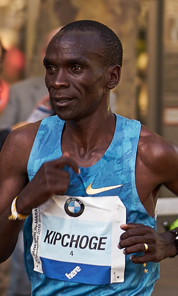
Figure: The Kapchorwa District, home district of Stephen Kiprotich.

Stephen Kiprotich, the 2012 gold medal winner from the London Olympics, comes from Kapchorwa district, in eastern Uganda, near the border with Kenya.

The common standard for collecting health data on the African continent is from the Health management information systems (HMIS). However, this data suffers from missing values (Gething et al., 2006) and diagnosis of diseases like typhoid and malaria may be confounded.

Figure: The Tororo district, where the sentinel site, Nagongera, is located.

World Health Organization Sentinel Surveillance systems are set up “when high-quality data are needed about a particular disease that cannot be obtained through a passive system.” Several sentinel sites give accurate assessment of malaria disease levels in Uganda, including a site in Nagongera.

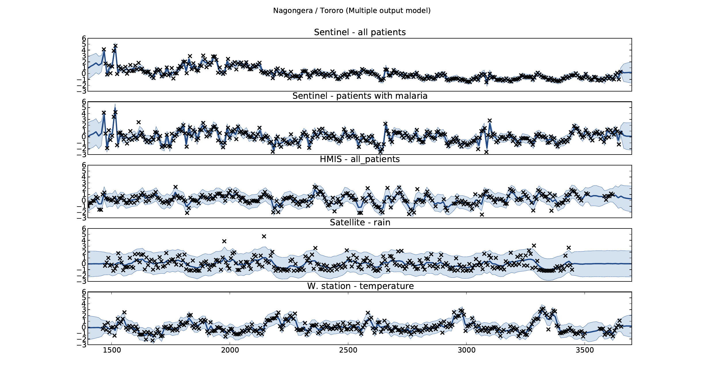
Figure: Sentinel and HMIS data along with rainfall and temperature for the Nagongera sentinel station in the Tororo district.

In collaboration with the AI Research Group at Makerere we chose to investigate whether Gaussian process models could be used to assimilate information from these two different sources of disease informaton. Further, we were interested in whether local information on rainfall and temperature could be used to improve malaria estimates.

The aim of the project was to use WHO Sentinel sites, alongside rainfall and temperature, to improve predictions from HMIS data of levels of malaria.

Figure: The Mubende District.

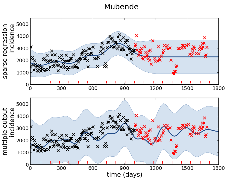
Figure: Prediction of malaria incidence in Mubende.

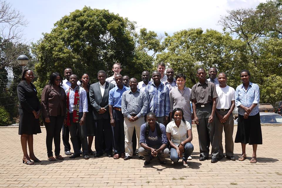
Figure: The project arose out of the Gaussian process summer school held at Makerere in Kampala in 2013. The school led, in turn, to the Data Science Africa initiative.

Early Warning Systems

Figure: The Kabarole district in Uganda.

Figure: Estimate of the current disease situation in the Kabarole district over time. Estimate is constructed with a Gaussian process with an additive covariance funciton.

Health monitoring system for the Kabarole district. Here we have fitted the reports with a Gaussian process with an additive covariance function. It has two components, one is a long time scale component (in red above) the other is a short time scale component (in blue).

Monitoring proceeds by considering two aspects of the curve. Is the blue line (the short term report signal) above the red (which represents the long term trend? If so we have higher than expected reports. If this is the case and the gradient is still positive (i.e. reports are going up) we encode this with a red color. If it is the case and the gradient of the blue line is negative (i.e. reports are going down) we encode this with an amber color. Conversely, if the blue line is below the red and decreasing, we color green. On the other hand if it is below red but increasing, we color yellow.

This gives us an early warning system for disease. Red is a bad situation getting worse, amber is bad, but improving. Green is good and getting better and yellow good but degrading.

Finally, there is a gray region which represents when the scale of the effect is small.

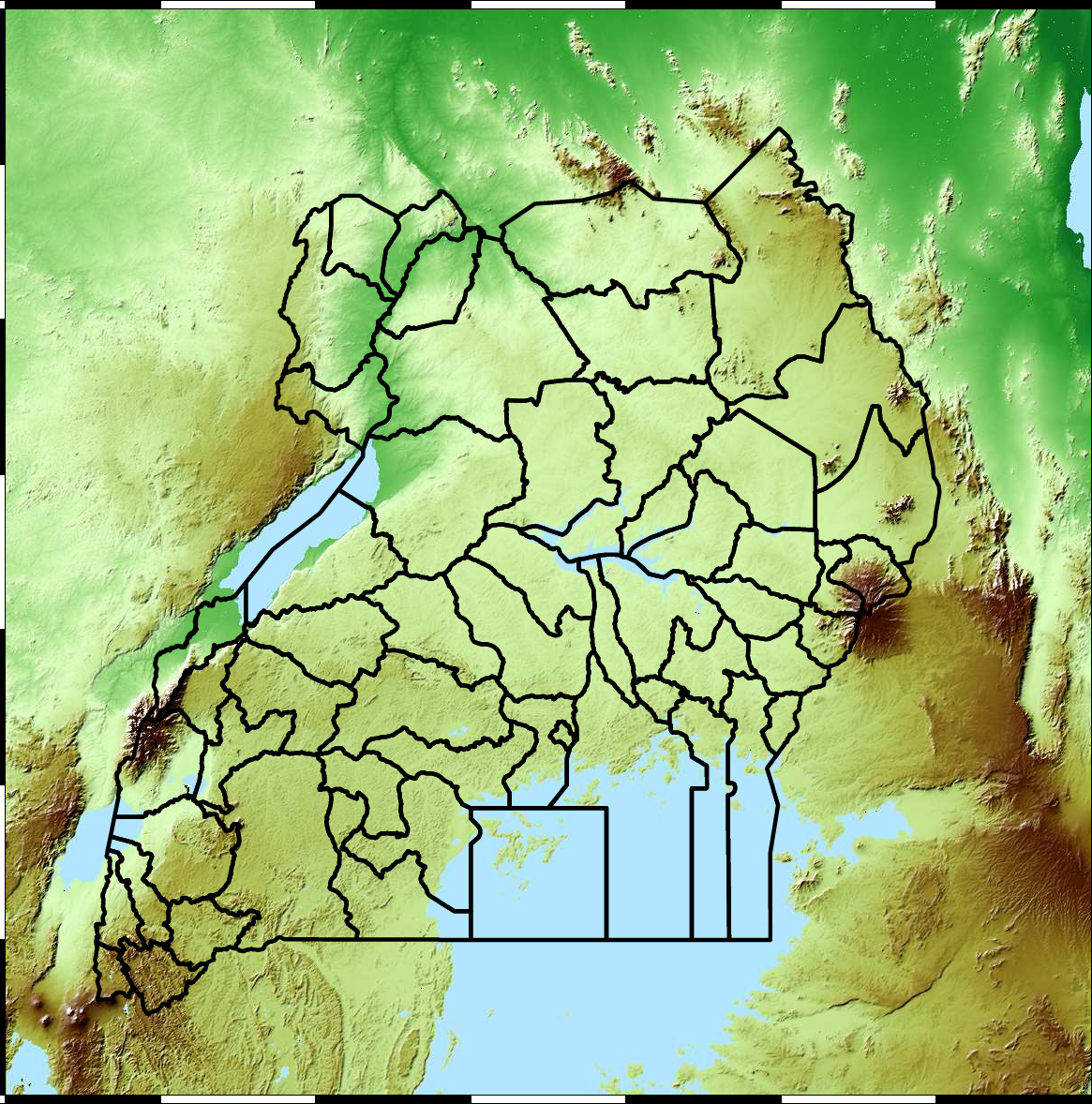
Figure: The map of Ugandan districts with an overview of the Malaria situation in each district.

These colors can now be observed directly on a spatial map of the districts to give an immediate impression of the current status of the disease across the country.

Additive Covariance

An additive covariance function is derived from considering the result of summing two Gaussian processes together. If the first Gaussian process is \(g(\cdot)\), governed by covariance \(k_g(\cdot, \cdot)\) and the second process is \(h(\cdot)\), governed by covariance \(k_h(\cdot, \cdot)\) then the combined process \(f(\cdot) = g(\cdot) + h(\cdot)\) is govererned by a covariance function, \[ k_f(\mathbf{ x}, \mathbf{ x}^\prime) = k_g(\mathbf{ x}, \mathbf{ x}^\prime) + k_h(\mathbf{ x}, \mathbf{ x}^\prime) \]

Figure: An additive covariance function formed by combining a linear and an exponentiated quadratic covariance functions.

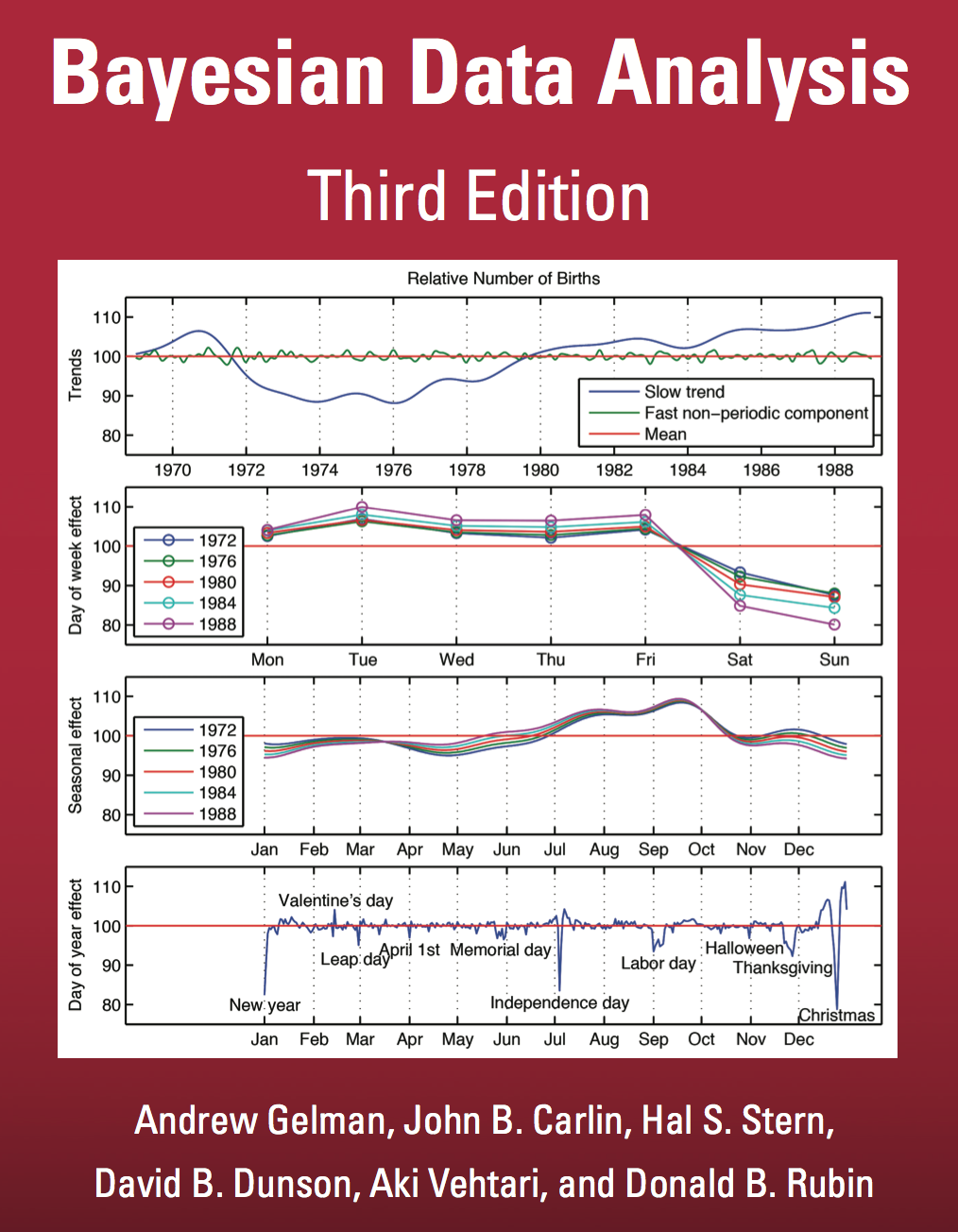
Analysis of US Birth Rates

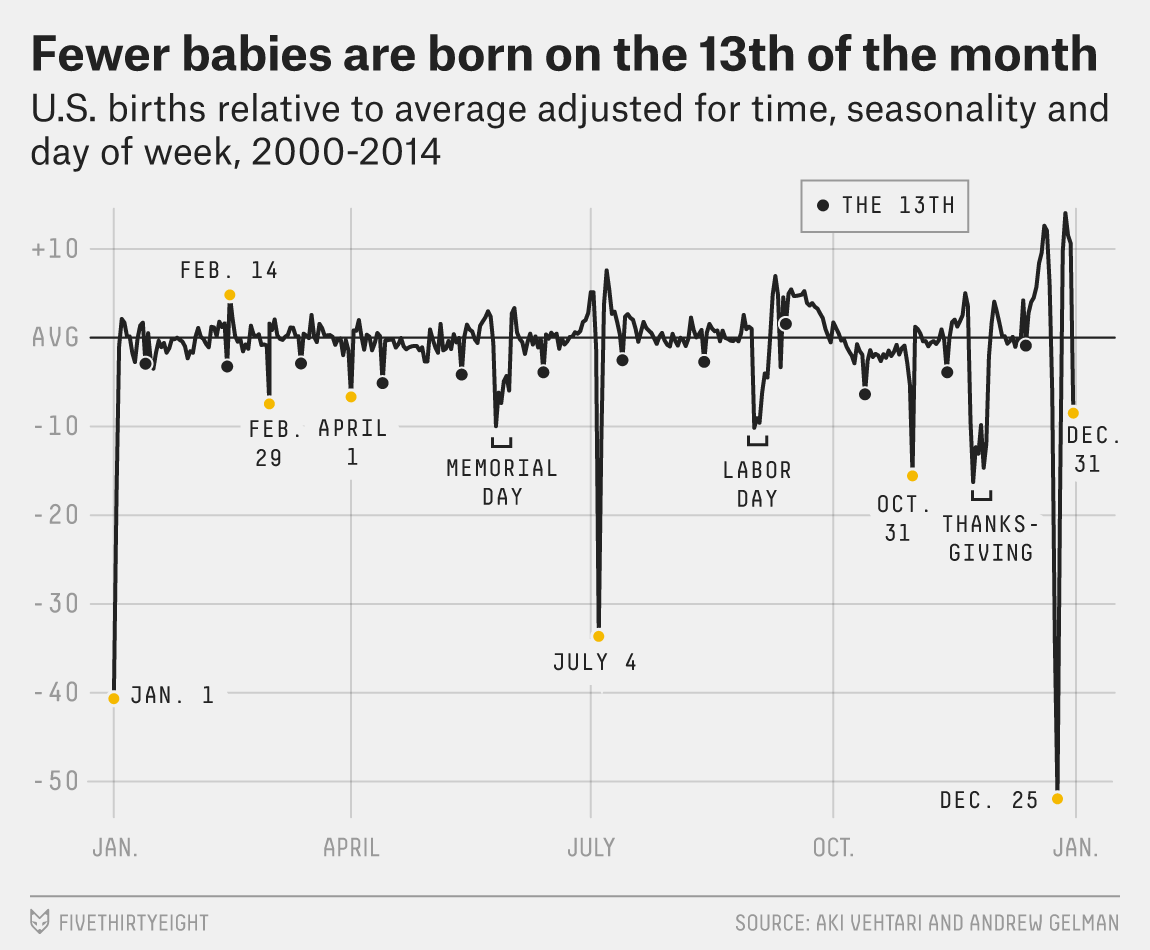
Figure: This is a retrospective analysis of US births by Aki Vehtari. The challenges of forecasting. Even with seasonal and weekly effects removed there are significant effects on holidays, weekends, etc.

There’s a nice analysis of US birth rates by Gaussian processes with additive covariances in Gelman et al. (2013). A combination of covariance functions are used to take account of weekly and yearly trends. The analysis is summarized on the cover of the book.

Figure: Two different editions of Bayesian Data Analysis (Gelman et al., 2013).

Basis Function Covariance

The fixed basis function covariance just comes from the properties of a multivariate Gaussian, if we decide \[ \mathbf{ f}=\boldsymbol{ \Phi}\mathbf{ w} \] and then we assume \[ \mathbf{ w}\sim \mathscr{N}\left(\mathbf{0},\alpha\mathbf{I}\right) \] then it follows from the properties of a multivariate Gaussian that \[ \mathbf{ f}\sim \mathscr{N}\left(\mathbf{0},\alpha\boldsymbol{ \Phi}\boldsymbol{ \Phi}^\top\right) \] meaning that the vector of observations from the function is jointly distributed as a Gaussian process and the covariance matrix is \(\mathbf{K}= \alpha\boldsymbol{ \Phi}\boldsymbol{ \Phi}^\top\), each element of the covariance matrix can then be found as the inner product between two rows of the basis funciton matrix.

from mlai import basis_cov

from mlai import radial

Figure: A covariance function based on a non-linear basis given by \(\boldsymbol{ \phi}(\mathbf{ x})\).

Brownian Covariance

from mlai import brownian_cov

Brownian motion is also a Gaussian process. It follows a Gaussian random walk, with diffusion occuring at each time point driven by a Gaussian input. This implies it is both Markov and Gaussian. The covariance function for Brownian motion has the form \[ k(t, t^\prime)=\alpha \min(t, t^\prime) \]

Figure: Brownian motion covariance function.

MLP Covariance

from mlai import mlp_cov

The multi-layer perceptron (MLP) covariance, also known as the neural network covariance or the arcsin covariance, is derived by considering the infinite limit of a neural network.

Figure: The multi-layer perceptron covariance function. This is derived by considering the infinite limit of a neural network with probit activation functions.

RELU Covariance

from mlai import relu_cov

Figure: Rectified linear unit covariance function.

Sinc Covariance

Another approach to developing covariance function exploits Bochner’s theorem (Bochner:book59?). Bochner’s theorem tells us that any positve filter in Fourier space implies has an associated Gaussian process with a stationary covariance function. The covariance function is the inverse Fourier transform of the filter applied in Fourier space.

For example, in signal processing, band limitations are commonly applied as an assumption. For example, we may believe that no frequency above \(w=2\) exists in the signal. This is equivalent to a rectangle function being applied as a the filter in Fourier space.

The inverse Fourier transform of the rectangle function is the \(\text{sinc}(\cdot)\) function. So the sinc is a valid covariance function, and it represents band limited signals.

Note that other covariance functions we’ve introduced can also be interpreted in this way. For example, the exponentiated quadratic covariance function can be Fourier transformed to see what the implied filter in Fourier space is. The Fourier transform of the exponentiated quadratic is an exponentiated quadratic, so the standard EQ-covariance implies a EQ filter in Fourier space.

from mlai import sinc_cov

Figure: Sinc covariance function.

Polynomial Covariance

Figure: Polynomial covariance function.

Periodic Covariance

Figure: Periodic covariance function.

Intrinsic Coregionalization Model Covariance

from mlai import icm_cov

Figure: Intrinsic coregionalization model covariance function.

Linear Model of Coregionalization Covariance

from mlai import lmc_cov

Figure: Linear model of coregionalization covariance function.

Semi Parametric Latent Factor Covariance

from mlai import icm_cov

from mlai import slfm_cov

import mlai.plot as plot
import mlai
import numpy as np

kernel = mlai.Kernel(function=mlai.slfm_cov, subkernel=mlai.eq_cov, W=np.asarray([[1],[5]]))

GPSS: Gaussian Process Summer School

If you’re interested in finding out more about Gaussian processes, you can attend the Gaussian process summer school, or view the lectures and material on line. Details of the school, future events and past events can be found at the website http://gpss.cc.

GPy: A Gaussian Process Framework in Python

Gaussian processes are a flexible tool for non-parametric analysis with uncertainty. The GPy software was started in Sheffield to provide a easy to use interface to GPs. One which allowed the user to focus on the modelling rather than the mathematics.

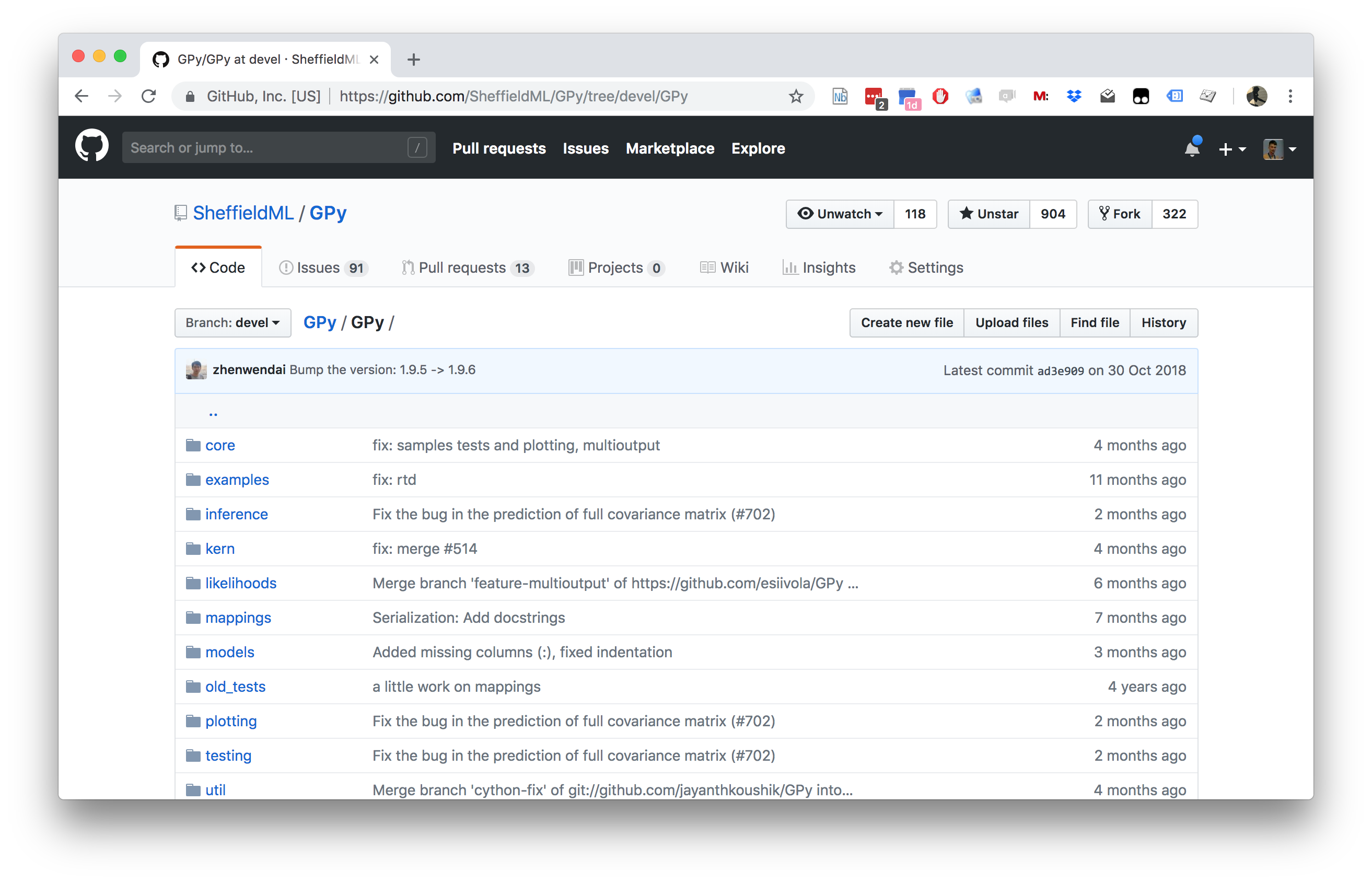
Figure: GPy is a BSD licensed software code base for implementing Gaussian process models in Python. It is designed for teaching and modelling. We welcome contributions which can be made through the GitHub repository https://github.com/SheffieldML/GPy

GPy is a BSD licensed software code base for implementing Gaussian process models in python. This allows GPs to be combined with a wide variety of software libraries.

The software itself is available on GitHub and the team welcomes contributions.

The aim for GPy is to be a probabilistic-style programming language, i.e., you specify the model rather than the algorithm. As well as a large range of covariance functions the software allows for non-Gaussian likelihoods, multivariate outputs, dimensionality reduction and approximations for larger data sets.

The documentation for GPy can be found here.

Further Reading

• Chapter 2 of Neal (1994)

• Rest of Neal (1994)

• All of MacKay (1992)

Thanks!

For more information on these subjects and more you might want to check the following resources.

• company: Trent AI
• book: The Atomic Human
• twitter: @lawrennd
• podcast: The Talking Machines
• newspaper: Guardian Profile Page
• blog: http://inverseprobability.com

References