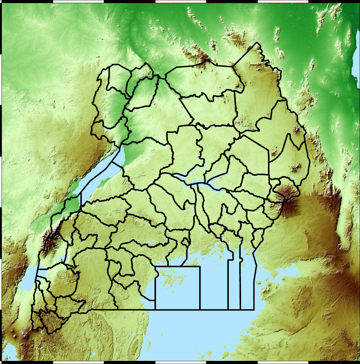
Andrade-Pacheco, R., Mubangizi, M., Quinn, J., Lawrence, N.D., 2014. Consistent mapping of government malaria records across a changing territory delimitation. Malaria Journal 13.
https://doi.org/10.1186/1475-2875-13-S1-P5
Della Gatta, G., Bansal, M., Ambesi-Impiombato, A., Antonini, D., Missero, C., Bernardo, D. di, 2008. Direct targets of the TRP63 transcription factor revealed by a combination of gene expression profiling and reverse engineering. Genome Research 18, 939–948.
https://doi.org/10.1101/gr.073601.107
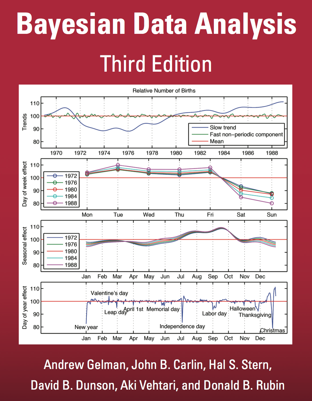
Gelman, A., Carlin, J.B., Stern, H.S., Dunson, D.B., Vehtari, A., Rubin, D.B., 2013. Bayesian data analysis, 3rd ed. Chapman; Hall.
Kalaitzis, A.A., Lawrence, N.D., 2011. A simple approach to ranking differentially expressed gene expression time courses through
Gaussian process regression. BMC Bioinformatics 12.
https://doi.org/10.1186/1471-2105-12-180
MacKay, D.J.C., 1992. Bayesian methods for adaptive models (PhD thesis). California Institute of Technology.
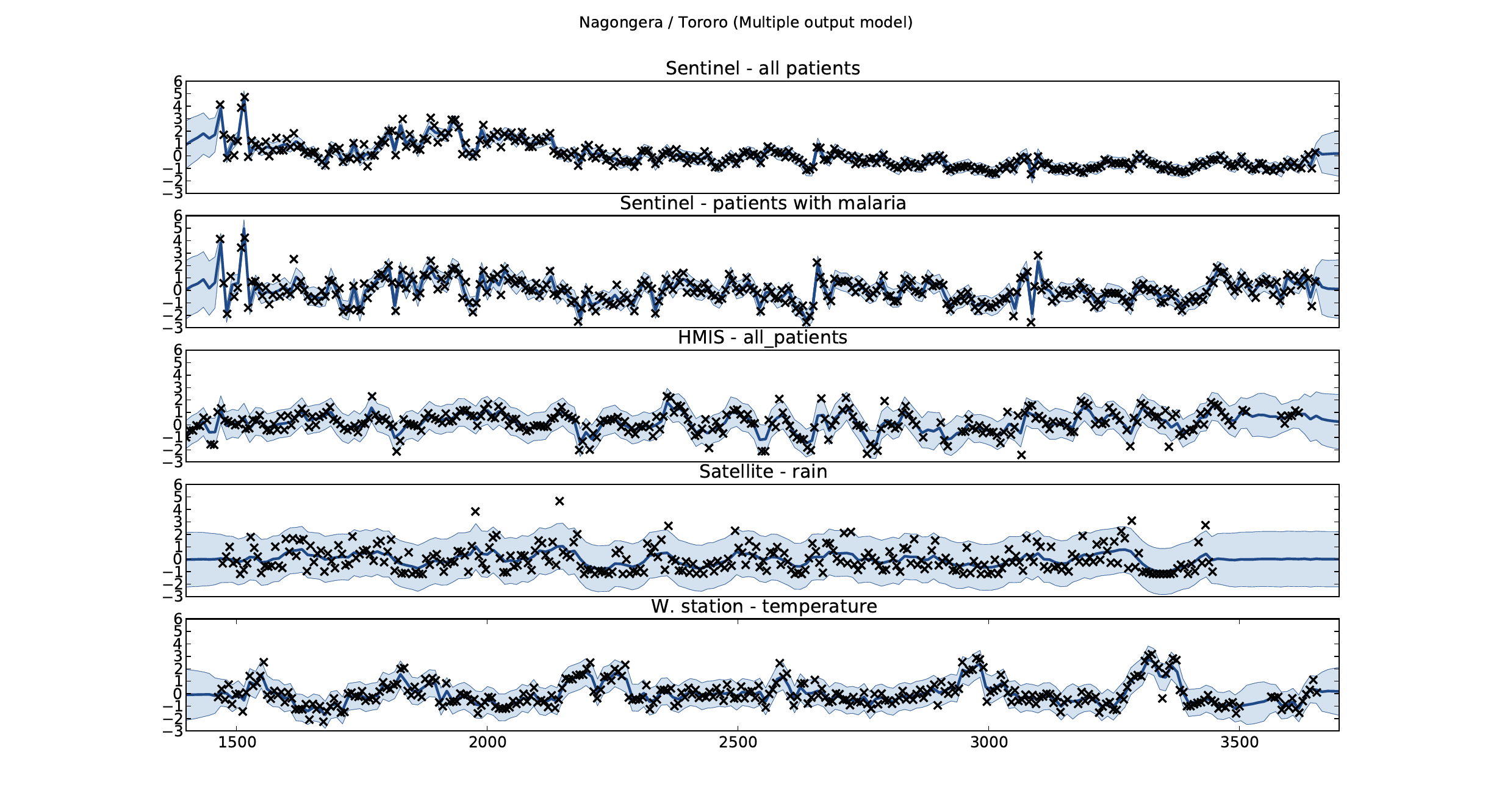
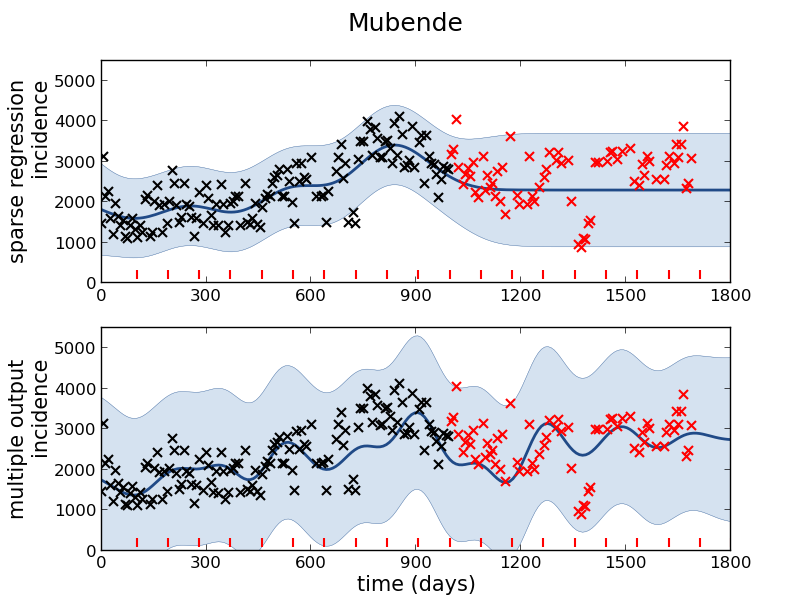
Mubangizi, M., Andrade-Pacheco, R., Smith, M.T., Quinn, J., Lawrence, N.D., 2014. Malaria surveillance with multiple data sources using Gaussian process models, in: 1st International Conference on the Use of Mobile ICT in Africa.
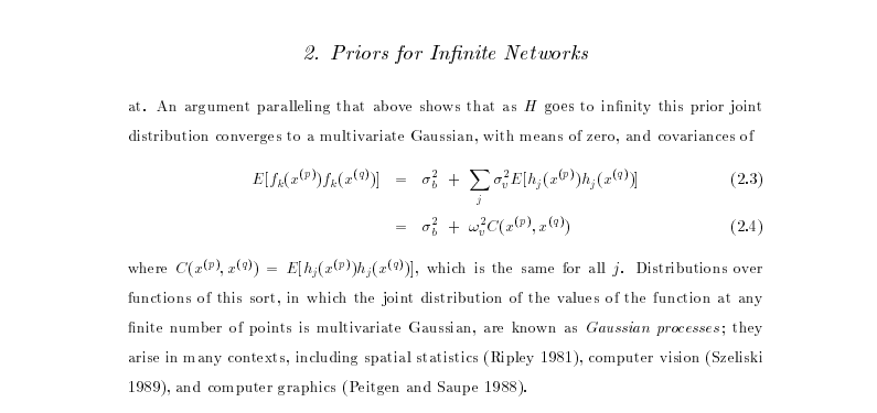
Neal, R.M., 1994. Bayesian learning for neural networks (PhD thesis). Dept. of Computer Science, University of Toronto.
Stein, M.L., 1999. Interpolation of spatial data: Some theory for Kriging. springer.

.jpg)