Week 10: Probabilistic Classification: Naive Bayes

[Powerpoint][jupyter][google colab][reveal]

Abstract: In the last lecture we looked at unsupervised learning. We introduced latent variables, dimensionality reduction and clustering. In this lecture we’re going to look at clustering, specifically the probabilistic approach to clustering. We’ll focus on a simple but often effective algorithm known as naive Bayes.

Setup

notutils

This small package is a helper package for various notebook utilities used below.

The software can be installed using

%pip install notutils

from the command prompt where you can access your python installation.

The code is also available on GitHub: https://github.com/lawrennd/notutils

Once notutils is installed, it can be imported in the usual manner.

import notutils

pods

In Sheffield we created a suite of software tools for ‘Open Data Science’. Open data science is an approach to sharing code, models and data that should make it easier for companies, health professionals and scientists to gain access to data science techniques.

You can also check this blog post on Open Data Science.

The software can be installed using

%pip install pods

from the command prompt where you can access your python installation.

The code is also available on GitHub: https://github.com/lawrennd/ods

Once pods is installed, it can be imported in the usual manner.

import pods

mlai

The mlai software is a suite of helper functions for teaching and demonstrating machine learning algorithms. It was first used in the Machine Learning and Adaptive Intelligence course in Sheffield in 2013.

The software can be installed using

%pip install mlai

from the command prompt where you can access your python installation.

The code is also available on GitHub: https://github.com/lawrennd/mlai

Once mlai is installed, it can be imported in the usual manner.

import mlai

Introduction to Classification

Classification is perhaps the technique most closely assocated with machine learning. In the speech based agents, on-device classifiers are used to determine when the wake word is used. A wake word is a word that wakes up the device. For the Amazon Echo it is “Alexa”, for Siri it is “Hey Siri”. Once the wake word detected with a classifier, the speech can be uploaded to the cloud for full processing, the speech recognition stages.

This isn’t just useful for intelligent agents, the UN global pulse project on public discussion on radio also uses wake word detection for recording radio conversations.

A major breakthrough in image classification came in 2012 with the ImageNet result of Alex Krizhevsky, Ilya Sutskever and Geoff Hinton from the University of Toronto. ImageNet is a large data base of 14 million images with many thousands of classes. The data is used in a community-wide challenge for object categorization. Krizhevsky et al used convolutional neural networks to outperform all previous approaches on the challenge. They formed a company which was purchased shortly after by Google. This challenge, known as object categorisation, was a major obstacle for practical computer vision systems. Modern object categorization systems are close to human performance.

Machine learning problems normally involve a prediction function and an objective function. Regression is the case where the prediction function iss over the real numbers, so the codomain of the functions, \(f(\mathbf{X})\) was the real numbers or sometimes real vectors. The classification problem consists of predicting whether or not a particular example is a member of a particular class. So we may want to know if a particular image represents a digit 6 or if a particular user will click on a given advert. These are classification problems, and they require us to map to yes or no answers. That makes them naturally discrete mappings.

In classification we are given an input vector, \(\mathbf{ x}\), and an associated label, \(y\) which either takes the value \(-1\) to represent no or \(1\) to represent yes.

In supervised learning the inputs, \(\mathbf{ x}\), are mapped to a label, \(y\), through a function \(f(\cdot)\) that is dependent on a set of parameters, \(\mathbf{ w}\), \[ y= f(\mathbf{ x}; \mathbf{ w}). \] The function \(f(\cdot)\) is known as the prediction function. The key challenges are (1) choosing which features, \(\mathbf{ x}\), are relevant in the prediction, (2) defining the appropriate class of function, \(f(\cdot)\), to use and (3) selecting the right parameters, \(\mathbf{ w}\).

Classification Examples

• Classifiying hand written digits from binary images (automatic zip code reading)
• Detecting faces in images (e.g. digital cameras).
• Who a detected face belongs to (e.g. Facebook, DeepFace)
• Classifying type of cancer given gene expression data.
• Categorization of document types (different types of news article on the internet)

Bernoulli Distribution

Our focus has been on models where the objective function is inspired by a probabilistic analysis of the problem. In particular we’ve argued that we answer questions about the data set by placing probability distributions over the various quantities of interest. For the case of binary classification this will normally involve introducing probability distributions for discrete variables. Such probability distributions, are in some senses easier than those for continuous variables, in particular we can represent a probability distribution over \(y\), where \(y\) is binary, with one value. If we specify the probability that \(y=1\) with a number that is between 0 and 1, i.e. let’s say that \(P(y=1) = \pi\) (here we don’t mean \(\pi\) the number, we are setting \(\pi\) to be a variable) then we can specify the probability distribution through a table.

Mathematically we can use a trick to implement this same table. We can use the value \(y\) as a mathematical switch and write that \[ P(y) = \pi^y(1-\pi)^{(1-y)} \] where our probability distribution is now written as a function of \(y\). This probability distribution is known as the Bernoulli distribution. The Bernoulli distribution is a clever trick for mathematically switching between two probabilities if we were to write it as code it would be better described as

def bernoulli(y_i, pi):
    if y_i == 1:
        return pi
    else:
        return 1-pi

If we insert \(y=1\) then the function is equal to \(\pi\), and if we insert \(y=0\) then the function is equal to \(1-\pi\). So the function recreates the table for the distribution given above.

The probability distribution is named for Jacob Bernoulli, the swiss mathematician. In his book Ars Conjectandi he considered the distribution and the result of a number of ‘trials’ under the Bernoulli distribution to form the binomial distribution. Below is the page where he considers Pascal’s triangle in forming combinations of the Bernoulli distribution to realise the binomial distribution for the outcome of positive trials.

Figure: Jacob Bernoulli described the Bernoulli distribution through an urn in which there are black and red balls.

Thomas Bayes also described the Bernoulli distribution, only he didn’t refer to Jacob Bernoulli’s work, so he didn’t call it by that name. He described the distribution in terms of a table (think of a billiard table) and two balls. Bayes suggests that each ball can be rolled across the table such that it comes to rest at a position that is uniformly distributed between the sides of the table.

Let’s assume that the first ball is rolled, and that it comes to reset at a position that is \(\pi\) times the width of the table from the left hand side.

Now, we roll the second ball. We are interested if the second ball ends up on the left side (+ve result) or the right side (-ve result) of the first ball. We use the Bernoulli distribution to determine this.

For this reason in Bayes’s distribution there is considered to be aleatoric uncertainty about the distribution parameter.

Figure: Thomas Bayes described the Bernoulli distribution independently of Jacob Bernoulli. He used the analogy of a billiard table. Any ball on the table is given a uniformly random position between the left and right side of the table. The first ball (in the figure) gives the parameter of the Bernoulli distribution. The second ball (in the figure) gives the outcome as either left or right (relative to the first ball). This is the origin of the term Bayesian because the parameter of the distribution is drawn from a probsbility.

Maximum Likelihood in the Bernoulli

Maximum likelihood in the Bernoulli distribution is straightforward. Let’s assume we have data, \(\mathbf{ y}\) which consists of a vector of binary values of length \(n\). If we assume each value was sampled independently from the Bernoulli distribution, conditioned on the parameter \(\pi\) then our joint probability density has the form \[ p(\mathbf{ y}|\pi) = \prod_{i=1}^{n} \pi^{y_i} (1-\pi)^{1-y_i}. \] As normal in maximum likelihood we consider the negative log likelihood as our objective, \[\begin{align*} E(\pi)& = -\log p(\mathbf{ y}|\pi)\\ & = -\sum_{i=1}^{n} y_i \log \pi - \sum_{i=1}^{n} (1-y_i) \log(1-\pi), \end{align*}\]

and we can derive the gradient with respect to the parameter \(\pi\). \[\frac{\text{d}E(\pi)}{\text{d}\pi} = -\frac{\sum_{i=1}^{n} y_i}{\pi} + \frac{\sum_{i=1}^{n} (1-y_i)}{1-\pi},\]

and as normal we look for a stationary point for the log likelihood by setting this derivative to zero, \[0 = -\frac{\sum_{i=1}^{n} y_i}{\pi} + \frac{\sum_{i=1}^{n} (1-y_i)}{1-\pi},\] rearranging we form \[(1-\pi)\sum_{i=1}^{n} y_i = \pi\sum_{i=1}^{n} (1-y_i),\] which implies \[\sum_{i=1}^{n} y_i = \pi\left(\sum_{i=1}^{n} (1-y_i) + \sum_{i=1}^{n} y_i\right),\]

and now we recognise that \(\sum_{i=1}^{n} (1-y_i) + \sum_{i=1}^{n} y_i = n\) so we have \[\pi = \frac{\sum_{i=1}^{n} y_i}{n}\]

so in other words we estimate the probability associated with the Bernoulli by setting it to the number of observed positives, divided by the total length of \(y\). This makes intiutive sense. If I asked you to estimate the probability of a coin being heads, and you tossed the coin 100 times, and recovered 47 heads, then the estimate of the probability of heads should be \(\frac{47}{100}\).

Exercise 1

Show that the maximum likelihood solution we have found is a minimum for our objective.

\[ \text{posterior} = \frac{\text{likelihood}\times\text{prior}}{\text{marginal likelihood}} \]

Four components:

1. Prior distribution
2. Likelihood
3. Posterior distribution
4. Marginal likelihood

Naive Bayes Classifiers

Note: Everything we do below is possible using standard packages like scikit-learn, our purpose in this session is to help you understand how those engines are constructed. In practice for an application you should use a library like scikit-learn.

In probabilistic machine learning we place probability distributions (or densities) over all the variables of interest, our first classification algorithm will do just that. We will consider how to form a classification by making assumptions about the joint density of our observations. We need to make assumptions to reduce the number of parameters we need to optimise.

In the ideal world, given label data \(\mathbf{ y}\) and the inputs \(\mathbf{X}\) we should be able to specify the joint density of all potential values of \(\mathbf{ y}\) and \(\mathbf{X}\), \(p(\mathbf{ y}, \mathbf{X})\). If \(\mathbf{X}\) and \(\mathbf{ y}\) are our training data, and we can somehow extend our density to incorporate future test data (by augmenting \(\mathbf{ y}\) with a new observation \(y^*\) and \(\mathbf{X}\) with the corresponding inputs, \(\mathbf{ x}^*\)), then we can answer any given question about a future test point \(y^*\) given its covariates \(\mathbf{ x}^*\) by conditioning on the training variables to recover, \[ p(y^*|\mathbf{X}, \mathbf{ y}, \mathbf{ x}^*), \]

We can compute this distribution using the product and sum rules. However, to specify this density we must give the probability associated with all possible combinations of \(\mathbf{ y}\) and \(\mathbf{X}\). There are \(2^{n}\) possible combinations for the vector \(\mathbf{ y}\) and the probability for each of these combinations must be jointly specified along with the joint density of the matrix \(\mathbf{X}\), as well as being able to extend the density for any chosen test location \(\mathbf{ x}^*\).

In naive Bayes we make certain simplifying assumptions that allow us to perform all of the above in practice.

Data Conditional Independence

If we are given model parameters \(\boldsymbol{ \theta}\) we assume that conditioned on all these parameters that all data points in the model are independent. In other words we have, \[ p(y^*, \mathbf{ x}^*, \mathbf{ y}, \mathbf{X}|\boldsymbol{ \theta}) = p(y^*, \mathbf{ x}^*|\boldsymbol{ \theta})\prod_{i=1}^{n} p(y_i, \mathbf{ x}_i | \boldsymbol{ \theta}). \] This is a conditional independence assumption because we are not assuming our data are purely independent. If we were to assume that, then there would be nothing to learn about our test data given our training data. We are assuming that they are independent given our parameters, \(\boldsymbol{ \theta}\). We made similar assumptions for regression, where our parameter set included \(\mathbf{ w}\) and \(\sigma^2\). Given those parameters we assumed that the density over \(\mathbf{ y}, y^*\) was independent. Here we are going a little further with that assumption because we are assuming the joint density of \(\mathbf{ y}\) and \(\mathbf{X}\) is independent across the data given the parameters.

Computing posterior distribution in this case becomes easier, this is known as the ‘Bayes classifier’.

Feature Conditional Independence

\[ p(\mathbf{ x}_i | y_i, \boldsymbol{ \theta}) = \prod_{j=1}^{p} p(x_{i,j}|y_i, \boldsymbol{ \theta}) \] where \(p\) is the dimensionality of our inputs.

The assumption that is particular to naive Bayes is to now consider that the features are also conditionally independent, but not only given the parameters. We assume that the features are independent given the parameters and the label. So for each data point we have \[p(\mathbf{ x}_i | y_i, \boldsymbol{ \theta}) = \prod_{j=1}^{p} p(x_{i,j}|y_i,\boldsymbol{ \theta})\] where \(p\) is the dimensionality of our inputs.

Marginal Density for \(y_i\)

\[ p(x_{i,j},y_i| \boldsymbol{ \theta}) = p(x_{i,j}|y_i, \boldsymbol{ \theta})p(y_i). \]

We now have nearly all of the components we need to specify the full joint density. However, the feature conditional independence doesn’t yet give us the joint density over \(p(y_i, \mathbf{ x}_i)\) which is required to subsitute in to our data conditional independence to give us the full density. To recover the joint density given the conditional distribution of each feature, \(p(x_{i,j}|y_i, \boldsymbol{ \theta})\), we need to make use of the product rule and combine it with a marginal density for \(y_i\),

\[p(x_{i,j},y_i| \boldsymbol{ \theta}) = p(x_{i,j}|y_i, \boldsymbol{ \theta})p(y_i).\] Because \(y_i\) is binary the Bernoulli density makes a suitable choice for our prior over \(y_i\), \[p(y_i|\pi) = \pi^{y_i} (1-\pi)^{1-y_i}\] where \(\pi\) now has the interpretation as being the prior probability that the classification should be positive.

Joint Density for Naive Bayes

This allows us to write down the full joint density of the training data, \[ p(\mathbf{ y}, \mathbf{X}|\boldsymbol{ \theta}, \pi) = \prod_{i=1}^{n} \prod_{j=1}^{p} p(x_{i,j}|y_i, \boldsymbol{ \theta})p(y_i|\pi) \]

which can now be fit by maximum likelihood. As normal we form our objective as the negative log likelihood,

\[\begin{align*} E(\boldsymbol{ \theta}, \pi)& = -\log p(\mathbf{ y}, \mathbf{X}|\boldsymbol{ \theta}, \pi) \\ &= -\sum_{i=1}^{n} \sum_{j=1}^{p} \log p(x_{i, j}|y_i, \boldsymbol{ \theta}) - \sum_{i=1}^{n} \log p(y_i|\pi), \end{align*}\] which we note decomposes into two objective functions, one which is dependent on \(\pi\) alone and one which is dependent on \(\boldsymbol{ \theta}\) alone so we have, \[ E(\pi, \boldsymbol{ \theta}) = E(\boldsymbol{ \theta}) + E(\pi). \] Since the two objective functions are separately dependent on the parameters \(\pi\) and \(\boldsymbol{ \theta}\) we can minimize them independently. Firstly, minimizing the Bernoulli likelihood over the labels we have, \[ E(\pi) = -\sum_{i=1}^{n}\log p(y_i|\pi) = -\sum_{i=1}^{n} y_i \log \pi - \sum_{i=1}^{n} (1-y_i) \log (1-\pi) \] which we already minimized above recovering \[ \pi = \frac{\sum_{i=1}^{n} y_i}{n}. \]

We now need to minimize the objective associated with the conditional distributions for the features, \[ E(\boldsymbol{ \theta}) = -\sum_{i=1}^{n} \sum_{j=1}^{p} \log p(x_{i, j} |y_i, \boldsymbol{ \theta}), \] which necessarily implies making some assumptions about the form of the conditional distributions. The right assumption will depend on the nature of our input data. For example, if we have an input which is real valued, we could use a Gaussian density and we could allow the mean and variance of the Gaussian to be different according to whether the class was positive or negative and according to which feature we were measuring. That would give us the form, \[ p(x_{i, j} | y_i,\boldsymbol{ \theta}) = \frac{1}{\sqrt{2\pi \sigma_{y_i,j}^2}} \exp \left(-\frac{(x_{i,j} - \mu_{y_i, j})^2}{\sigma_{y_i,j}^2}\right), \] where \(\sigma_{1, j}^2\) is the variance of the density for the \(j\)th output and the class \(y_i=1\) and \(\sigma_{0, j}^2\) is the variance if the class is 0. The means can vary similarly. Our parameters, \(\boldsymbol{ \theta}\) would consist of all the means and all the variances for the different dimensions.

As normal we form our objective as the negative log likelihood, \[ E(\boldsymbol{ \theta}, \pi) = -\log p(\mathbf{ y}, \mathbf{X}|\boldsymbol{ \theta}, \pi) = -\sum_{i=1}^{n} \sum_{j=1}^{p} \log p(x_{i, j}|y_i, \boldsymbol{ \theta}) - \sum_{i=1}^{n} \log p(y_i|\pi), \] which we note decomposes into two objective functions, one which is dependent on \(\pi\) alone and one which is dependent on \(\boldsymbol{ \theta}\) alone so we have, \[ E(\pi, \boldsymbol{ \theta}) = E(\boldsymbol{ \theta}) + E(\pi). \]

Nigeria NMIS Data

As an example data set we will use Nigerian Millennium Development Goals Information System Health Facility (The Office of the Senior Special Assistant to the President on the Millennium Development Goals (OSSAP-MDGs) and Columbia University, 2014). It can be found here https://energydata.info/dataset/nigeria-nmis-education-facility-data-2014.

Taking from the information on the site,

The Nigeria MDG (Millennium Development Goals) Information System – NMIS health facility data is collected by the Office of the Senior Special Assistant to the President on the Millennium Development Goals (OSSAP-MDGs) in partner with the Sustainable Engineering Lab at Columbia University. A rigorous, geo-referenced baseline facility inventory across Nigeria is created spanning from 2009 to 2011 with an additional survey effort to increase coverage in 2014, to build Nigeria’s first nation-wide inventory of health facility. The database includes 34,139 health facilities info in Nigeria.

The goal of this database is to make the data collected available to planners, government officials, and the public, to be used to make strategic decisions for planning relevant interventions.

For data inquiry, please contact Ms. Funlola Osinupebi, Performance Monitoring & Communications, Advisory Power Team, Office of the Vice President at funlola.osinupebi@aptovp.org

To learn more, please visit http://csd.columbia.edu/2014/03/10/the-nigeria-mdg-information-system-nmis-takes-open-data-further/

Suggested citation: Nigeria NMIS facility database (2014), the Office of the Senior Special Assistant to the President on the Millennium Development Goals (OSSAP-MDGs) & Columbia University

For ease of use we’ve packaged this data set in the pods library

data = pods.datasets.nigeria_nmis()['Y']
data.head()

Alternatively, you can access the data directly with the following commands.

import urllib.request
urllib.request.urlretrieve('https://energydata.info/dataset/f85d1796-e7f2-4630-be84-79420174e3bd/resource/6e640a13-cab4-457b-b9e6-0336051bac27/download/healthmopupandbaselinenmisfacility.csv', 'healthmopupandbaselinenmisfacility.csv')

import pandas as pd
data = pd.read_csv('healthmopupandbaselinenmisfacility.csv')

Once it is loaded in the data can be summarized using the describe method in pandas.

data.describe()

We can also find out the dimensions of the dataset using the shape property.

data.shape

Dataframes have different functions that you can use to explore and understand your data. In python and the Jupyter notebook it is possible to see a list of all possible functions and attributes by typing the name of the object followed by .<Tab> for example in the above case if we type data.<Tab> it show the columns available (these are attributes in pandas dataframes) such as num_nurses_fulltime, and also functions, such as .describe().

For functions we can also see the documentation about the function by following the name with a question mark. This will open a box with documentation at the bottom which can be closed with the x button.

data.describe?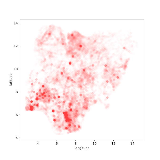

Figure: Location of the over thirty-four thousand health facilities registered in the NMIS data across Nigeria. Each facility plotted according to its latitude and longitude.

Nigeria NMIS Data Classification

Our aim will be to predict whether a center has maternal health delivery services given the attributes in the data. We will predict of the number of nurses, the number of doctors, location etc.

Now we will convert this data into a form which we can use as inputs X, and labels y.

import pandas as pd
import numpy as np

data = data[~pd.isnull(data['maternal_health_delivery_services'])]
data = data.dropna() # Remove entries with missing values
X = data[['emergency_transport',
          'num_chews_fulltime', 
          'phcn_electricity',
          'child_health_measles_immun_calc',
          'num_nurses_fulltime',
          'num_doctors_fulltime', 
          'improved_water_supply', 
          'improved_sanitation',
          'antenatal_care_yn', 
          'family_planning_yn',
          'malaria_treatment_artemisinin', 
          'latitude', 
          'longitude']].copy()
y = data['maternal_health_delivery_services']==True  # set label to be whether there's a maternal health delivery service

# Create series of health center types with the relevant index
s = data['facility_type_display'].apply(pd.Series, 1).stack() 
s.index = s.index.droplevel(-1) # to line up with df's index

# Extract from the series the unique list of types.
types = s.unique()

# For each type extract the indices where it is present and add a column to X
type_names = []
for htype in types:
    index = s[s==htype].index.tolist()
    type_col=htype.replace(' ', '_').replace('/','-').lower()
    type_names.append(type_col)
    X.loc[:, type_col] = 0.0 
    X.loc[index, type_col] = 1.0

This has given us a new data frame X which contains the different facility types in different columns.

X.describe()

Naive Bayes NMIS

We can now specify the naive Bayes model. For the genres we want to model the data as Bernoulli distributed, and for the year and body count we want to model the data as Gaussian distributed. We set up two data frames to contain the parameters for the rows and the columns below.

# assume data is binary or real.
# this list encodes whether it is binary or real (1 for binary, 0 for real)
binary_columns = ['emergency_transport',
          'phcn_electricity',
          'child_health_measles_immun_calc',
          'improved_water_supply', 
          'improved_sanitation',
          'antenatal_care_yn', 
          'family_planning_yn',
          'malaria_treatment_artemisinin'] + type_names
real_columns = ['num_chews_fulltime', 
                'num_nurses_fulltime', 
                'num_doctors_fulltime', 
                'latitude', 
                'longitude']
Bernoulli = pd.DataFrame(data=np.zeros((2,len(binary_columns))), columns=binary_columns, index=['theta_0', 'theta_1'])
Gaussian = pd.DataFrame(data=np.zeros((4,len(real_columns))), columns=real_columns, index=['mu_0', 'sigma2_0', 'mu_1', 'sigma2_1'])

Now we have the data in a form ready for analysis, let’s construct our data matrix.

num_train = 20000
indices = np.random.permutation(X.shape[0])
train_indices = indices[:num_train]
test_indices = indices[num_train:]
X_train = X.iloc[train_indices]
y_train = y.iloc[train_indices]==True
X_test = X.iloc[test_indices]
y_test = y.iloc[test_indices]==True

And we can now train the model. For each feature we can make the fit independently. The fit is given by either counting the number of positives (for binary data) which gives us the maximum likelihood solution for the Bernoulli. Or by computing the empirical mean and variance of the data for the Gaussian, which also gives us the maximum likelihood solution.

for column in X_train:
    if column in Gaussian:
        Gaussian[column]['mu_0'] = X_train[column][~y_train].mean()
        Gaussian[column]['mu_1'] = X_train[column][y_train].mean()
        Gaussian[column]['sigma2_0'] = X_train[column][~y_train].var(ddof=0)
        Gaussian[column]['sigma2_1'] = X_train[column][y_train].var(ddof=0)
    if column in Bernoulli:
        Bernoulli[column]['theta_0'] = X_train[column][~y_train].sum()/(~y_train).sum()
        Bernoulli[column]['theta_1'] = X_train[column][y_train].sum()/(y_train).sum()

We can examine the nature of the distributions we’ve fitted to the model by looking at the entries in these data frames.

Bernoulli

The distributions show the parameters of the independent class conditional probabilities for no maternity services. It is a Bernoulli distribution with the parameter, \(\pi\), given by (theta_0) for the facilities without maternity services and theta_1 for the facilities with maternity services. The parameters whow that, facilities with maternity services also are more likely to have other services such as grid electricity, emergency transport, immunization programs etc.

The naive Bayes assumption says that the joint probability for these services is given by the product of each of these Bernoulli distributions.

Gaussian

We have modelled the numbers in our table with a Gaussian density. Since several of these numbers are counts, a more appropriate distribution might be the Poisson distribution. But here we can see that the average number of nurses, healthworkers and doctors is higher in the facilities with maternal services (mu_1) than those without maternal services (mu_0). There is also a small difference between the mean latitude and longitudes. However, the standard deviation which would be given by the square root of the variance parameters (sigma_0 and sigma_1) is large, implying that a difference in latitude and longitude may be due to sampling error. To be sure more analysis would be required.

The final model parameter is the prior probability of the positive class, \(\pi\), which is computed by maximum likelihood.

prior = float(y_train.sum())/len(y_train)

The prior probability tells us that slightly more facilities have maternity services than those that don’t.

Making Predictions

Naive Bayes has given us the class conditional densities: \(p(\mathbf{ x}_i | y_i, \boldsymbol{ \theta})\). To make predictions with these densities we need to form the distribution given by \[ P(y^*| \mathbf{ y}, \mathbf{X}, \mathbf{ x}^*, \boldsymbol{ \theta}) \] This can be computed by using the product rule. We know that \[ P(y^*| \mathbf{ y}, \mathbf{X}, \mathbf{ x}^*, \boldsymbol{ \theta})p(\mathbf{ y}, \mathbf{X}, \mathbf{ x}^*|\boldsymbol{ \theta}) = p(y*, \mathbf{ y}, \mathbf{X}, \mathbf{ x}^*| \boldsymbol{ \theta}) \] implying that \[ P(y^*| \mathbf{ y}, \mathbf{X}, \mathbf{ x}^*, \boldsymbol{ \theta}) = \frac{p(y*, \mathbf{ y}, \mathbf{X}, \mathbf{ x}^*| \boldsymbol{ \theta})}{p(\mathbf{ y}, \mathbf{X}, \mathbf{ x}^*|\boldsymbol{ \theta})} \] and we’ve already defined \(p(y^*, \mathbf{ y}, \mathbf{X}, \mathbf{ x}^*| \boldsymbol{ \theta})\) using our conditional independence assumptions above \[ p(y^*, \mathbf{ y}, \mathbf{X}, \mathbf{ x}^*| \boldsymbol{ \theta}) = \prod_{j=1}^{p} p(x^*_{j}|y^*, \boldsymbol{ \theta})p(y^*|\pi)\prod_{i=1}^{n} \prod_{j=1}^{p} p(x_{i,j}|y_i, \boldsymbol{ \theta})p(y_i|\pi) \] The other required density is \[ p(\mathbf{ y}, \mathbf{X}, \mathbf{ x}^*|\boldsymbol{ \theta}) \] which can be found from \[p(y^*, \mathbf{ y}, \mathbf{X}, \mathbf{ x}^*| \boldsymbol{ \theta})\] using the sum rule of probability, \[ p(\mathbf{ y}, \mathbf{X}, \mathbf{ x}^*|\boldsymbol{ \theta}) = \sum_{y^*=0}^1 p(y^*, \mathbf{ y}, \mathbf{X}, \mathbf{ x}^*| \boldsymbol{ \theta}). \] Because of our independence assumptions that is simply equal to \[ p(\mathbf{ y}, \mathbf{X}, \mathbf{ x}^*| \boldsymbol{ \theta}) = \sum_{y^*=0}^1 \prod_{j=1}^{p} p(x^*_{j}|y^*_i, \boldsymbol{ \theta})p(y^*|\pi)\prod_{i=1}^{n} \prod_{j=1}^{p} p(x_{i,j}|y_i, \boldsymbol{ \theta})p(y_i|\pi). \] Substituting both forms in to recover our distribution over the test label conditioned on the training data we have, \[ P(y^*| \mathbf{ y}, \mathbf{X}, \mathbf{ x}^*, \boldsymbol{ \theta}) = \frac{\prod_{j=1}^{p} p(x^*_{j}|y^*_i, \boldsymbol{ \theta})p(y^*|\pi)\prod_{i=1}^{n} \prod_{j=1}^{p} p(x_{i,j}|y_i, \boldsymbol{ \theta})p(y_i|\pi)}{\sum_{y^*=0}^1 \prod_{j=1}^{p} p(x^*_{j}|y^*_i, \boldsymbol{ \theta})p(y^*|\pi)\prod_{i=1}^{n} \prod_{j=1}^{p} p(x_{i,j}|y_i, \boldsymbol{ \theta})p(y_i|\pi)} \] and we notice that all the terms associated with the training data actually cancel, the test prediction is conditionally independent of the training data given the parameters. This is a result of our conditional independence assumptions over the data points. \[ p(y^*| \mathbf{ x}^*, \boldsymbol{ \theta}) = \frac{\prod_{j=1}^{p} p(x^*_{j}|y^*_i, \boldsymbol{ \theta})p(y^*|\pi)}{\sum_{y^*=0}^1 \prod_{j=1}^{p} p(x^*_{j}|y^*_i, \boldsymbol{ \theta})p(y^*|\pi)} \] This formula is also fairly straightforward to implement. First we implement the log probabilities for the Gaussian density.

def log_gaussian(x, mu, sigma2):
    return -0.5* np.log(2*np.pi*sigma2)-((x-mu)**2)/(2*sigma2)

Now for any test point we compute the joint distribution of the Gaussian features by summing their log probabilities. Working in log space can be a considerable advantage over computing the probabilities directly: as the number of features we include goes up, because all the probabilities are less than 1, the joint probability will become smaller and smaller, and may be difficult to represent accurately (or even underflow). Working in log space can ameliorate this problem. We can also compute the log probability for the Bernoulli distribution.

def log_bernoulli(x, theta):
    return x*np.log(theta) + (1-x)*np.log(1-theta)

Laplace Smoothing

Before we proceed, let’s just pause and think for a moment what will happen if theta here is either zero or one. This will result in \(\log 0 = -\infty\) and cause numerical problems. This definitely can happen in practice. If some of the features are rare or very common across the data set then the maximum likelihood solution could find values of zero or one respectively. Such values are problematic because they cause posterior probabilities of class membership of either one or zero. In practice we deal with this using Laplace smoothing (which actually has an interpretation as a Bayesian fit of the Bernoulli distribution. Laplace used an example of the sun rising each day, and a wish to predict the sun rise the following day to describe his idea of smoothing, which can be found at the bottom of following page from Laplace’s ‘Essai Philosophique …’

Laplace suggests that when computing the probability of an event where a success or failure is rare (he uses an example of the sun rising across the last 5,000 years or 1,826,213 days) that even though only successes have been observed (in the sun rising case) that the odds for tomorrow shouldn’t be given as \[ \frac{1,826,213}{1,826,213} = 1 \] but rather by adding one to the numerator and two to the denominator, \[ \frac{1,826,213 + 1}{1,826,213 + 2} = 0.99999945. \] This technique is sometimes called a ‘pseudocount technique’ because it has an intepretation of assuming some observations before you start, it’s as if instead of observing \(\sum_{i}y_i\) successes you have an additional success, \(\sum_{i}y_i + 1\) and instead of having observed \(n\) events you’ve observed \(n+ 2\). So we can think of Laplace’s idea saying (before we start) that we have ‘two observations worth of belief, that the odds are 50/50’, because before we start (i.e. when \(n=0\)) our estimate is 0.5, yet because the effective \(n\) is only 2, this estimate is quickly overwhelmed by data. Laplace used ideas like this a lot, and it is known as his ‘principle of insufficient reason’. His idea was that in the absence of knowledge (i.e. before we start) we should assume that all possible outcomes are equally likely. This idea has a modern counterpart, known as the principle of maximum entropy. A lot of the theory of this approach was developed by Ed Jaynes, who according to his erstwhile collaborator and friend, John Skilling, learnt French as an undergraduate by reading the works of Laplace. Although John also related that Jaynes’s spoken French was not up to the standard of his scientific French. For me Ed Jaynes’s work very much carries on the tradition of Laplace into the modern era, in particular his focus on Bayesian approaches. I’m very proud to have met those that knew and worked with him. It turns out that Laplace’s idea also has a Bayesian interpretation (as Laplace understood), it comes from assuming a particular prior density for the parameter \(\pi\), but we won’t explore that interpretation for the moment, and merely choose to estimate the probability as, \[ \pi = \frac{\sum_{i=1}^{n} y_i + 1}{n+ 2} \] to prevent problems with certainty causing numerical issues and misclassifications. Let’s refit the Bernoulli features now.

# fit the Bernoulli with Laplace smoothing.
for column in X_train:
    if column in Bernoulli:
        Bernoulli[column]['theta_0'] = (X_train[column][~y_train].sum() + 1)/((~y_train).sum() + 2)
        Bernoulli[column]['theta_1'] = (X_train[column][y_train].sum() + 1)/((y_train).sum() + 2)

That places us in a position to write the prediction function.

import numpy as np
import pandas as pd

def predict(X_test, Gaussian, Bernoulli, prior):
    log_positive = pd.Series(data = np.zeros(X_test.shape[0]), index=X_test.index)
    log_negative = pd.Series(data = np.zeros(X_test.shape[0]), index=X_test.index)
    for column in X_test.columns:
        if column in Gaussian:
            log_positive += log_gaussian(X_test[column], Gaussian[column]['mu_1'], Gaussian[column]['sigma2_1'])
            log_negative += log_gaussian(X_test[column], Gaussian[column]['mu_0'], Gaussian[column]['sigma2_0'])
        elif column in Bernoulli:
            log_positive += log_bernoulli(X_test[column], Bernoulli[column]['theta_1'])
            log_negative += log_bernoulli(X_test[column], Bernoulli[column]['theta_0'])
            
    v = np.zeros_like(log_positive.values)
    for i in range(X_test.shape[0]):
        v[i] = np.exp(log_positive.values[i] + np.log(prior))/(np.exp(log_positive.values[i] + np.log(prior)) 
                                                               + np.exp(log_negative.values[i] + np.log(1-prior)))
    return v
    #return np.exp(log_positive + np.log(prior))/(np.exp(log_positive + np.log(prior)) + np.exp(log_negative + np.log(1-prior)))

Now we are in a position to make the predictions for the test data.

p_y = predict(X_test, Gaussian, Bernoulli, prior)

We can test the quality of the predictions in the following way. Firstly, we can threshold our probabilities at 0.5, allocating points with greater than 50% probability of membership of the positive class to the positive class. We can then compare to the true values, and see how many of these values we got correct. This is our total number correct.

correct = y_test.eq(p_y>0.5)
total_correct = sum(correct)
print("Total correct", total_correct, " out of ", len(y_test), "which is", float(total_correct)/len(y_test), "%")

We can also now plot the confusion matrix. A confusion matrix tells us where we are making mistakes. Along the diagonal it stores the true positives, the points that were positive class that we classified correctly, and the true negatives, the points that were negative class and that we classified correctly. The off diagonal terms contain the false positives and the false negatives. Along the rows of the matrix we place the actual class, and along the columns we place our predicted class.

confusion_matrix = pd.DataFrame(data=np.zeros((2,2)), 
                                columns=['predicted no maternity', 'predicted maternity'],
                                index =['actual no maternity','actual maternity'])
confusion_matrix['predicted maternity']['actual maternity'] = (y_test & (p_y>0.5)).sum()
confusion_matrix['predicted maternity']['actual no maternity'] = (~y_test & (p_y>0.5)).sum()
confusion_matrix['predicted no maternity']['actual maternity'] = (y_test & ~(p_y>0.5)).sum()
confusion_matrix['predicted no maternity']['actual no maternity'] = (~y_test & ~(p_y>0.5)).sum()
confusion_matrix

Exercise 2

How can you improve your classification, are all the features equally valid? Are some features more helpful than others? What happens if you remove features that appear to be less helpful. How might you select such features?

Exercise 3

We have decided to classify positive if probability of maternity is greater than 0.5. This has led us to accidentally classify some facilities as havien’t facilities for maternity when in fact they don’t. Imagine you wish to ensure that a facility handles maternity. With your test set how low do you have to set the threshold to avoid all the false negatives (i.e. facilities where you predicted there was no maternity, but in actuality there were?

Making Predictions

Naive Bayes has given us the class conditional densities: \(p(\mathbf{ x}_i | y_i, \boldsymbol{ \theta})\). To make predictions with these densities we need to form the distribution given by \[ P(y^*| \mathbf{ y}, \mathbf{X}, \mathbf{ x}^*, \boldsymbol{ \theta}) \]

Exercise 4

Write down the negative log likelihood of the Gaussian density over a vector of variables \(\mathbf{ x}\). Assume independence between each variable. Minimize this objective to obtain the maximum likelihood solution of the form. \[ \mu = \frac{\sum_{i=1}^{n} x_i}{n} \] \[ \sigma^2 = \frac{\sum_{i=1}^{n} (x_i - \mu)^2}{n} \]

If the input data was binary then we could also make use of the Bernoulli distribution for the features. For that case we would have the form, \[ p(x_{i, j} | y_i,\boldsymbol{ \theta}) = \theta_{y_i, j}^{x_{i, j}}(1-\theta_{y_i, j})^{(1-x_{i,j})}, \] where \(\theta_{1, j}\) is the probability that the \(j\)th feature is on if \(y_i\) is 1.

In either case, maximum likelihood fitting would proceed in the same way. The objective has the form, \[ E(\boldsymbol{ \theta}) = -\sum_{j=1}^{p} \sum_{i=1}^{n} \log p(x_{i,j} |y_i, \boldsymbol{ \theta}), \] and if, as above, the parameters of the distributions are specific to each feature vector (we had means and variances for each continuous feature, and a probability for each binary feature) then we can use the fact that these parameters separate into disjoint subsets across the features to write, \[ \begin{align*} E(\boldsymbol{ \theta}) &= -\sum_{j=1}^{p} \sum_{i=1}^{n} \log p(x_{i,j} |y_i, \boldsymbol{ \theta}_j)\\ & \sum_{j=1}^{p} E(\boldsymbol{ \theta}_j), \end{align*} \] which means we can minimize our objective on each feature independently.

These characteristics mean that naive Bayes scales very well with big data. To fit the model we consider each feature in turn, we select the positive class and fit parameters for that class, then we select each negative class and fit features for that class. We have code below.

Naive Bayes Summary

Naive Bayes is making very simple assumptions about the data, in particular it is modeling the full joint probability of the data set, \(p(\mathbf{ y}, \mathbf{X}| \boldsymbol{ \theta}, \pi)\) by very strong assumptions about factorizations that are unlikely to be true in practice. The data conditional independence assumption is common, and relies on a rich parameter vector to absorb all the information in the training data. The additional assumption of naive Bayes is that features are conditional independent given the class label \(y_i\) (and the parameter vector, \(\boldsymbol{ \theta}\). This is quite a strong assumption. However, it causes the objective function to decompose into parts which can be independently fitted to the different feature vectors, meaning it is very easy to fit the model to large data. It is also clear how we should handle streaming data and missing data. This means that the model can be run ‘live’, adapting parameters and information as it arrives. Indeed, the model is even capable of dealing with new features that might arrive at run time. Such is the strength of the modeling the joint probability density. However, the factorization assumption that allows us to do this efficiently is very strong and may lead to poor decision boundaries in practice.

Further Reading

• Chapter 5 up to pg 179 (Section 5.1, and 5.2 up to 5.2.2) of Rogers and Girolami (2011)

Thanks!

For more information on these subjects and more you might want to check the following resources.

• twitter: @lawrennd
• podcast: The Talking Machines
• newspaper: Guardian Profile Page
• blog: http://inverseprobability.com

References