Probabilistic Classification: Naive Bayes
Review
- Last time: Looked at unsupervised learning.
- Introduced latent variables, dimensionality reduction and clustering.
- This time: Classification with Naive Bayes
Introduction to Classification
Classification
Wake word classification (Global Pulse Project).
Breakthrough in 2012 with ImageNet result of Alex Krizhevsky, Ilya Sutskever and Geoff Hinton
We are given a data set containing ‘inputs’, \(\mathbf{X}\) and ‘targets’, \(\mathbf{ y}\).
Each data point consists of an input vector \(\mathbf{ x}_i\) and a class label, \(y_i\).
For binary classification assume \(y_i\) should be either \(1\) (yes) or \(-1\) (no).
Input vector can be thought of as features.
Discrete Probability
- Algorithms based on prediction function and objective function.
- For regression the codomain of the functions, \(f(\mathbf{X})\) was the real numbers or sometimes real vectors.
- In classification we are given an input vector, \(\mathbf{ x}\), and an associated label, \(y\) which either takes the value \(-1\) or \(1\).
Classification
- Inputs, \(\mathbf{ x}\), mapped to a label, \(y\), through a function \(f(\cdot)\) dependent on parameters, \(\mathbf{ w}\), \[ y= f(\mathbf{ x}; \mathbf{ w}). \]
- \(f(\cdot)\) is known as the prediction function.
Classification Examples
- Classifiying hand written digits from binary images (automatic zip code reading)
- Detecting faces in images (e.g. digital cameras).
- Who a detected face belongs to (e.g. Facebook, DeepFace)
- Classifying type of cancer given gene expression data.
- Categorization of document types (different types of news article on the internet)
Reminder on the Term “Bayesian”
- We use Bayes’ rule to invert probabilities in the Bayesian approach.
- Bayesian is not named after Bayes’ rule (v. common confusion).
- The term Bayesian refers to the treatment of the parameters as stochastic variables.
- Proposed by Laplace (1774) and Bayes (1763) independently.
- For early statisticians this was very controversial (Fisher et al).
Reminder on the Term “Bayesian”
- The use of Bayes’ rule does not imply you are being
Bayesian.
- It is just an application of the product rule of probability.
Bernoulli Distribution
- Binary classification: need a probability distribution for discrete variables.
- Discrete probability is in some ways easier: \(P(y=1) = \pi\) & specify distribution as a table.
- Instead of \(y=-1\) for negative class we take \(y=0\).
| \(y\) | 0 | 1 |
|---|---|---|
| \(P(y)\) | \((1-\pi)\) | \(\pi\) |
This is the Bernoulli distribution.
Mathematical Switch
The Bernoulli distribution \[ P(y) = \pi^y(1-\pi)^{(1-y)} \]
Is a clever trick for switching probabilities, as code it would be
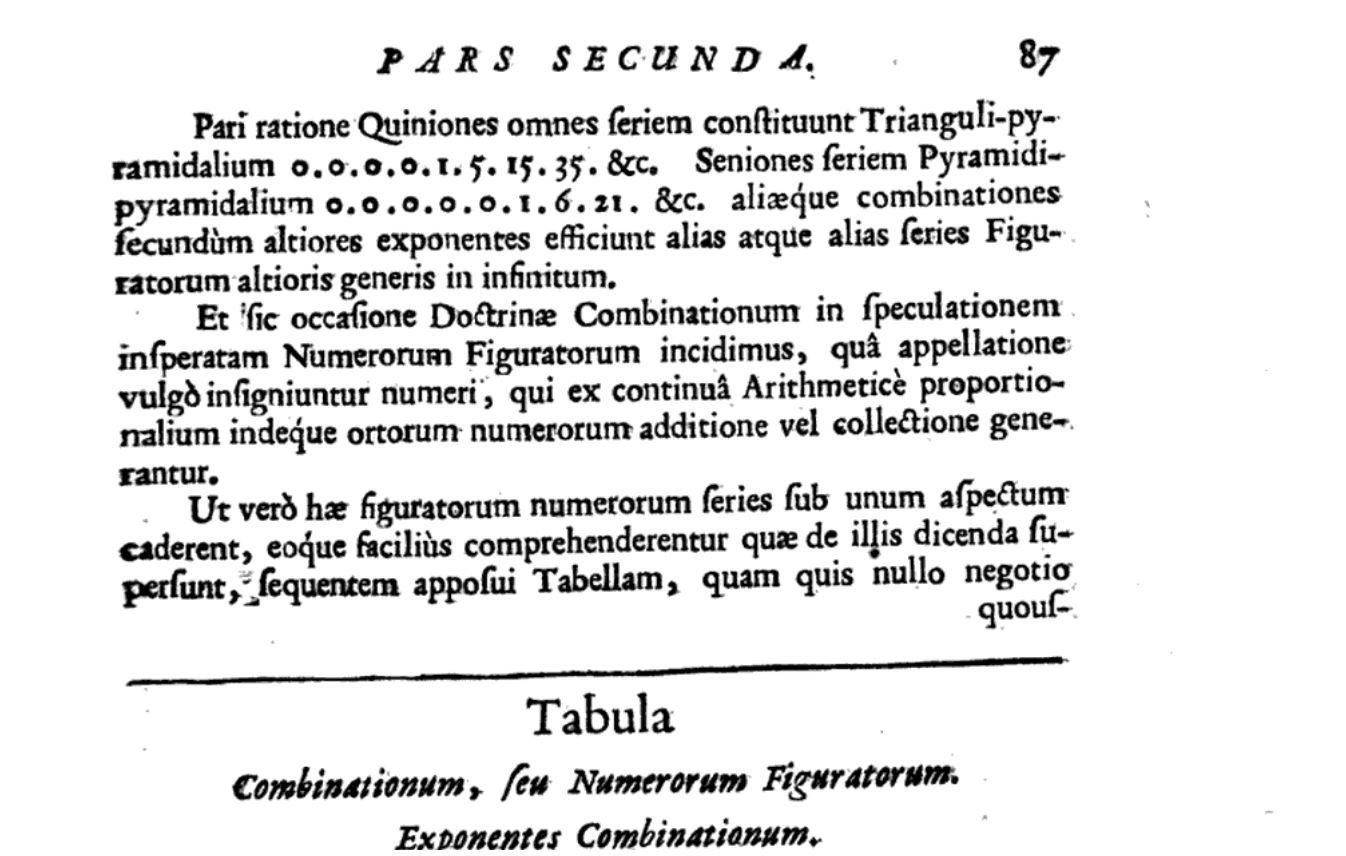
Jacob Bernoulli’s Bernoulli
- Bernoulli described the Bernoulli distribution in terms of an ‘urn’ filled with balls.
- There are red and black balls. There is a fixed number of balls in the urn.
- The portion of red balls is given by \(\pi\).
- For this reason in Bernoulli’s distribution there is epistemic uncertainty about the distribution parameter.
Jacob Bernoulli’s Bernoulli
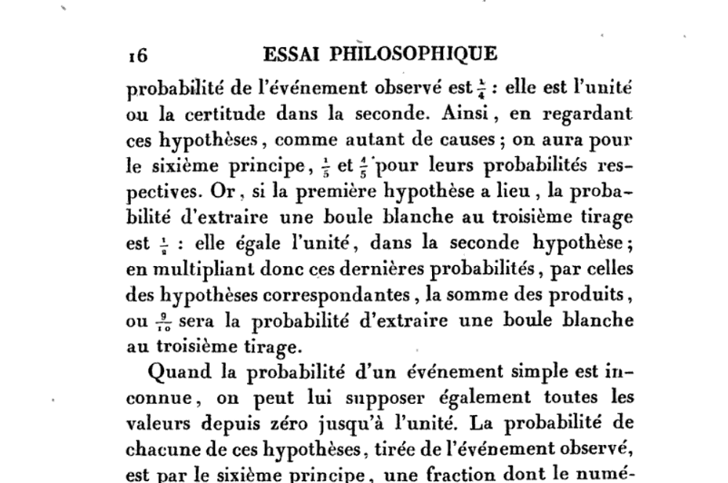
Thomas Bayes’s Bernoulli
- Bayes described the Bernoulli distribution (he didn’t call it that!) in terms of a table and two balls.
- Each ball is rolled so it comes to rest at a uniform distribution across the table.
- The first ball comes to rest at a position that is a \(\pi\) times the width of table.
- After placing the first ball you consider whether a second would land to the left or the right.
- For this reason in Bayes’s distribution there is considered to be aleatoric uncertainty about the distribution parameter.
Thomas Bayes’ Bernoulli
Maximum Likelihood in the Bernoulli
- Assume data, \(\mathbf{ y}\) is binary vector length \(n\).
- Assume each value was sampled independently from the Bernoulli distribution, given probability \(\pi\) \[ p(\mathbf{ y}|\pi) = \prod_{i=1}^{n} \pi^{y_i} (1-\pi)^{1-y_i}. \]
Negative Log Likelihood
- Minimize the negative log likelihood \[\begin{align*} E(\pi)& = -\log p(\mathbf{ y}|\pi)\\ & = -\sum_{i=1}^{n} y_i \log \pi - \sum_{i=1}^{n} (1-y_i) \log(1-\pi), \end{align*}\]
- Take gradient with respect to the parameter \(\pi\). \[\frac{\text{d}E(\pi)}{\text{d}\pi} = -\frac{\sum_{i=1}^{n} y_i}{\pi} + \frac{\sum_{i=1}^{n} (1-y_i)}{1-\pi},\]
Fixed Point
Stationary point: set derivative to zero \[0 = -\frac{\sum_{i=1}^{n} y_i}{\pi} + \frac{\sum_{i=1}^{n} (1-y_i)}{1-\pi},\]
Rearrange to form \[(1-\pi)\sum_{i=1}^{n} y_i = \pi\sum_{i=1}^{n} (1-y_i),\]
Giving \[\sum_{i=1}^{n} y_i = \pi\left(\sum_{i=1}^{n} (1-y_i) + \sum_{i=1}^{n} y_i\right),\]
Solution
Recognise that \(\sum_{i=1}^{n} (1-y_i) + \sum_{i=1}^{n} y_i = n\) so we have \[\pi = \frac{\sum_{i=1}^{n} y_i}{n}\]
Estimate the probability associated with the Bernoulli by setting it to the number of observed positives, divided by the total length of \(y\).
Makes intiutive sense.
What’s your best guess of probability for coin toss is heads when you get 47 heads from 100 tosses?
Bayes’ Rule Reminder
\[ \text{posterior} = \frac{\text{likelihood}\times\text{prior}}{\text{marginal likelihood}} \]
Four components:
- Prior distribution
- Likelihood
- Posterior distribution
- Marginal likelihood
Naive Bayes Classifiers
Probabilistic Machine Learning: place probability distributions (or densities) over all the variables of interest.
In naive Bayes this is exactly what we do.
Form a classification algorithm by modelling the joint density of our observations.
Need to make assumption about joint density.
Assumptions about Density
- Make assumptions to reduce the number of parameters we need to optimise.
- Given label data \(\mathbf{ y}\) and the inputs \(\mathbf{X}\) could specify joint density of all potential values of \(\mathbf{ y}\) and \(\mathbf{X}\), \(p(\mathbf{ y}, \mathbf{X})\).
- If \(\mathbf{X}\) and \(\mathbf{ y}\) are training data.
- If \(\mathbf{ x}^*\) is a test input and \(y^*\) a test location we want \[ p(y^*|\mathbf{X}, \mathbf{ y}, \mathbf{ x}^*), \]
Answer from Rules of Probability
- Compute this distribution using the product and sum rules.
- Need the probability associated with all possible combinations of \(\mathbf{ y}\) and \(\mathbf{X}\).
- There are \(2^{n}\) possible combinations for the vector \(\mathbf{ y}\)
- Probability for each of these combinations must be jointly specified along with the joint density of the matrix \(\mathbf{X}\),
- Also need to extend the density for any chosen test location \(\mathbf{ x}^*\).
Naive Bayes Assumptions
- In naive Bayes we make certain simplifying assumptions that allow us to perform all of the above in practice.
- Data Conditional Independence
- Feature conditional independence
- Marginal density for \(y\).
Data Conditional Independence
Given model parameters \(\boldsymbol{ \theta}\) we assume that all data points in the model are independent. \[ p(y^*, \mathbf{ x}^*, \mathbf{ y}, \mathbf{X}|\boldsymbol{ \theta}) = p(y^*, \mathbf{ x}^*|\boldsymbol{ \theta})\prod_{i=1}^{n} p(y_i, \mathbf{ x}_i | \boldsymbol{ \theta}). \]
This is a conditional independence assumption.
We also make similar assumptions for regression (where \(\boldsymbol{ \theta}= \left\{\mathbf{ w},\sigma^2\right\}\)).
Here we assume joint density of \(\mathbf{ y}\) and \(\mathbf{X}\) is independent across the data given the parameters.
Bayes Classifier
Computing posterior distribution in this case becomes easier, this is known as the ‘Bayes classifier’.
Feature Conditional Independence
- Particular to naive Bayes: assume features are also conditionally independent, given param and the label. \[p(\mathbf{ x}_i | y_i, \boldsymbol{ \theta}) = \prod_{j=1}^{p} p(x_{i,j}|y_i,\boldsymbol{ \theta})\] where \(p\) is the dimensionality of our inputs.
- This is known as the naive Bayes assumption.
- Bayes classifier + feature conditional independence.
Marginal Density for \(y_i\)
To specify the joint distribution we also need the marginal for \(p(y_i)\) \[p(x_{i,j},y_i| \boldsymbol{ \theta}) = p(x_{i,j}|y_i, \boldsymbol{ \theta})p(y_i).\]
Because \(y_i\) is binary the Bernoulli density makes a suitable choice for our prior over \(y_i\), \[p(y_i|\pi) = \pi^{y_i} (1-\pi)^{1-y_i}\] where \(\pi\) now has the interpretation as being the prior probability that the classification should be positive.
Joint Density for Naive Bayes
- This allows us to write down the full joint density of the training data, \[ p(\mathbf{ y}, \mathbf{X}|\boldsymbol{ \theta}, \pi) = \prod_{i=1}^{n} \prod_{j=1}^{p} p(x_{i,j}|y_i, \boldsymbol{ \theta})p(y_i|\pi) \] which can now be fit by maximum likelihood.
Objective Function
\[\begin{align*} E(\boldsymbol{ \theta}, \pi)& = -\log p(\mathbf{ y}, \mathbf{X}|\boldsymbol{ \theta}, \pi) \\ &= -\sum_{i=1}^{n} \sum_{j=1}^{p} \log p(x_{i, j}|y_i, \boldsymbol{ \theta}) - \sum_{i=1}^{n} \log p(y_i|\pi), \end{align*}\]
Maximum Likelihood
Fit Prior
- We can minimize prior. For Bernoulli likelihood over the labels we have, \[\begin{align*} E(\pi) & = - \sum_{i=1}^{n}\log p(y_i|\pi)\\ & = -\sum_{i=1}^{n} y_i \log \pi - \sum_{i=1}^{n} (1-y_i) \log (1-\pi) \end{align*}\]
- Solution from above is \[ \pi = \frac{\sum_{i=1}^{n} y_i}{n}. \]
Fit Conditional
- Minimize conditional distribution: \[ E(\boldsymbol{ \theta}) = -\sum_{i=1}^{n} \sum_{j=1}^{p} \log p(x_{i, j} |y_i, \boldsymbol{ \theta}), \]
- Implies making an assumption about it’s form.
- The right assumption will depend on the data.
- E.g. for real valued data, use a Gaussian \[ p(x_{i, j} | y_i,\boldsymbol{ \theta}) = \frac{1}{\sqrt{2\pi \sigma_{y_i,j}^2}} \exp \left(-\frac{(x_{i,j} - \mu_{y_i, j})^2}{\sigma_{y_i,j}^2}\right), \]
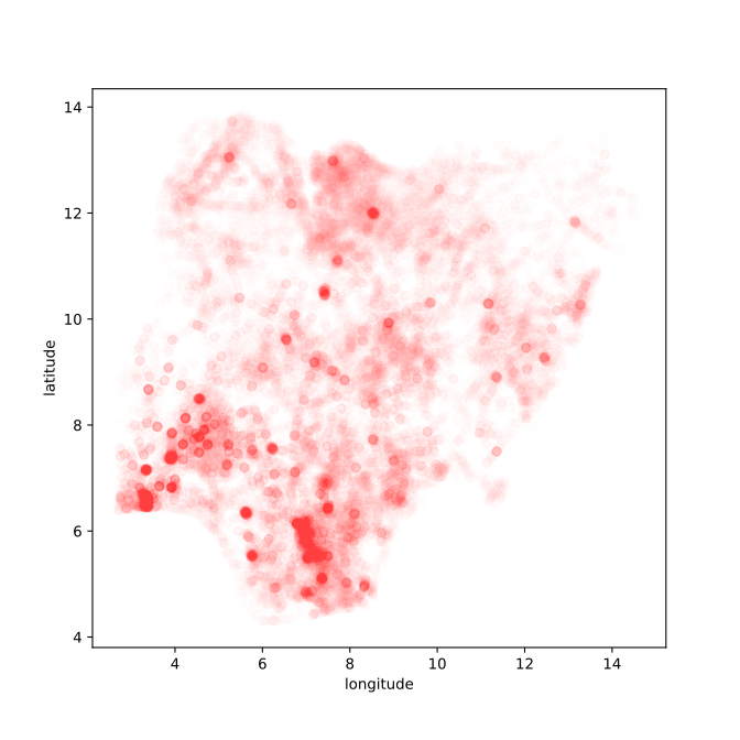
Nigeria NMIS Data
Nigeria NMIS Data: Notebook

Nigeria NMIS Data Classification
The distributions show the parameters of the independent
class conditional probabilities for no maternity services. It is a
Bernoulli distribution with the parameter, \(\pi\), given by (theta_0) for
the facilities without maternity services and theta_1 for
the facilities with maternity services. The parameters whow that,
facilities with maternity services also are more likely to have other
services such as grid electricity, emergency transport, immunization
programs etc.
The naive Bayes assumption says that the joint probability for these services is given by the product of each of these Bernoulli distributions.
We have modelled the numbers in our table with a Gaussian density.
Since several of these numbers are counts, a more appropriate
distribution might be the Poisson distribution. But here we can see that
the average number of nurses, healthworkers and doctors is
higher in the facilities with maternal services
(mu_1) than those without maternal services
(mu_0). There is also a small difference between the mean
latitude and longitudes. However, the standard deviation which
would be given by the square root of the variance parameters
(sigma_0 and sigma_1) is large, implying that
a difference in latitude and longitude may be due to sampling error. To
be sure more analysis would be required.
Compute Posterior for Test Point Label
- We know that \[ P(y^*| \mathbf{ y}, \mathbf{X}, \mathbf{ x}^*, \boldsymbol{ \theta})p(\mathbf{ y},\mathbf{X}, \mathbf{ x}^*|\boldsymbol{ \theta}) = p(y*, \mathbf{ y}, \mathbf{X},\mathbf{ x}^*| \boldsymbol{ \theta}) \]
- This implies \[ P(y^*| \mathbf{ y}, \mathbf{X}, \mathbf{ x}^*, \boldsymbol{ \theta}) = \frac{p(y*, \mathbf{ y}, \mathbf{X}, \mathbf{ x}^*| \boldsymbol{ \theta})}{p(\mathbf{ y}, \mathbf{X}, \mathbf{ x}^*|\boldsymbol{ \theta})} \]
Compute Posterior for Test Point Label
- From conditional independence assumptions \[ p(y^*, \mathbf{ y}, \mathbf{X}, \mathbf{ x}^*| \boldsymbol{ \theta}) = \prod_{j=1}^{p} p(x^*_{j}|y^*, \boldsymbol{ \theta})p(y^*|\pi)\prod_{i=1}^{n} \prod_{j=1}^{p} p(x_{i,j}|y_i, \boldsymbol{ \theta})p(y_i|\pi) \]
- We also need \[ p(\mathbf{ y}, \mathbf{X}, \mathbf{ x}^*|\boldsymbol{ \theta})\] which can be found from \[p(y^*, \mathbf{ y}, \mathbf{X}, \mathbf{ x}^*| \boldsymbol{ \theta}) \]
- Using the sum rule of probability, \[ p(\mathbf{ y}, \mathbf{X}, \mathbf{ x}^*|\boldsymbol{ \theta}) = \sum_{y^*=0}^1 p(y^*, \mathbf{ y}, \mathbf{X}, \mathbf{ x}^*| \boldsymbol{ \theta}). \]
Independence Assumptions
- From independence assumptions \[ p(\mathbf{ y}, \mathbf{X}, \mathbf{ x}^*| \boldsymbol{ \theta}) = \sum_{y^*=0}^1 \prod_{j=1}^{p} p(x^*_{j}|y^*_i, \boldsymbol{ \theta})p(y^*|\pi)\prod_{i=1}^{n} \prod_{j=1}^{p} p(x_{i,j}|y_i, \boldsymbol{ \theta})p(y_i|\pi). \]
- Substitute both forms to recover, \[ P(y^*| \mathbf{ y}, \mathbf{X}, \mathbf{ x}^*, \boldsymbol{ \theta}) = \frac{\prod_{j=1}^{p} p(x^*_{j}|y^*_i, \boldsymbol{ \theta})p(y^*|\pi)\prod_{i=1}^{n} \prod_{j=1}^{p} p(x_{i,j}|y_i, \boldsymbol{ \theta})p(y_i|\pi)}{\sum_{y^*=0}^1 \prod_{j=1}^{p} p(x^*_{j}|y^*_i, \boldsymbol{ \theta})p(y^*|\pi)\prod_{i=1}^{n} \prod_{j=1}^{p} p(x_{i,j}|y_i, \boldsymbol{ \theta})p(y_i|\pi)} \]
Cancelation
- Note training data terms cancel. \[ p(y^*| \mathbf{ x}^*, \boldsymbol{ \theta}) = \frac{\prod_{j=1}^{p} p(x^*_{j}|y^*_i, \boldsymbol{ \theta})p(y^*|\pi)}{\sum_{y^*=0}^1 \prod_{j=1}^{p} p(x^*_{j}|y^*_i, \boldsymbol{ \theta})p(y^*|\pi)} \]
- This formula is also fairly straightforward to implement for different class conditional distributions.
Laplace Smoothing
Pseudo Counts
\[ \pi = \frac{\sum_{i=1}^{n} y_i + 1}{n+ 2} \]
Naive Bayes Summary
- Model full joint distribution of data, \(p(\mathbf{ y}, \mathbf{X}| \boldsymbol{ \theta}, \pi)\)
- Make conditional independence assumptions about the data.
- feature conditional independence
- data conditional independence
- Fast to implement, works on very large data.
- Despite simple assumptions can perform better than expected.
Further Reading
- Chapter 5 up to pg 179 (Section 5.1, and 5.2 up to 5.2.2) of Rogers and Girolami (2011)
Thanks!
twitter: @lawrennd
podcast: The Talking Machines
newspaper: Guardian Profile Page
blog posts:

