

%pip install gpyGPy: A Gaussian Process Framework in Python
Gaussian processes are a flexible tool for non-parametric analysis with uncertainty. The GPy software was started in Sheffield to provide a easy to use interface to GPs. One which allowed the user to focus on the modelling rather than the mathematics.
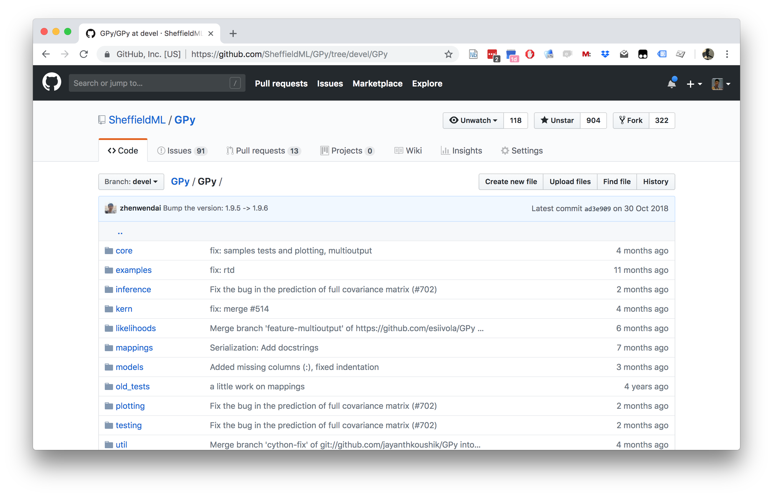

Figure: GPy is a BSD licensed software code base for implementing Gaussian process models in Python. It is designed for teaching and modelling. We welcome contributions which can be made through the GitHub repository https://github.com/SheffieldML/GPy
GPy is a BSD licensed software code base for implementing Gaussian process models in python. This allows GPs to be combined with a wide variety of software libraries.
The software itself is available on GitHub and the team welcomes contributions.
The aim for GPy is to be a probabilistic-style programming language, i.e., you specify the model rather than the algorithm. As well as a large range of covariance functions the software allows for non-Gaussian likelihoods, multivariate outputs, dimensionality reduction and approximations for larger data sets.
The documentation for GPy can be found here.
- GP-LVM Provides probabilistic non-linear dimensionality reduction.
- How to select the dimensionality?
- Need to estimate marginal likelihood.
- In standard GP-LVM it increases with increasing \(q\).
|
Bayesian GP-LVM
|
|
Standard Variational Approach Fails
- Standard variational bound has the form: \[ \mathcal{L}= \left\langle\log p(\mathbf{ y}|\mathbf{Z})\right\rangle_{q(\mathbf{Z})} + \text{KL}\left( q(\mathbf{Z})\,\|\,p(\mathbf{Z}) \right) \]
The standard variational approach would require the expectation of \(\log p(\mathbf{ y}|\mathbf{Z})\) under \(q(\mathbf{Z})\). \[ \begin{align} \log p(\mathbf{ y}|\mathbf{Z}) = & -\frac{1}{2}\mathbf{ y}^\top\left(\mathbf{K}_{\mathbf{ f}, \mathbf{ f}}+\sigma^2\mathbf{I}\right)^{-1}\mathbf{ y}\\ & -\frac{1}{2}\log \det{\mathbf{K}_{\mathbf{ f}, \mathbf{ f}}+\sigma^2 \mathbf{I}} -\frac{n}{2}\log 2\pi \end{align} \] But this is extremely difficult to compute because \(\mathbf{K}_{\mathbf{ f}, \mathbf{ f}}\) is dependent on \(\mathbf{Z}\) and it appears in the inverse.
Variational Bayesian GP-LVM
The alternative approach is to consider the collapsed variational bound (used for low rank (sparse is a misnomer) Gaussian process approximations. \[ p(\mathbf{ y})\geq \prod_{i=1}^nc_i \int \mathcal{N}\left(\mathbf{ y}|\left\langle\mathbf{ f}\right\rangle,\sigma^2\mathbf{I}\right)p(\mathbf{ u}) \text{d}\mathbf{ u} \] \[ p(\mathbf{ y}|\mathbf{Z})\geq \prod_{i=1}^nc_i \int \mathcal{N}\left(\mathbf{ y}|\left\langle\mathbf{ f}\right\rangle_{p(\mathbf{ f}|\mathbf{ u}, \mathbf{Z})},\sigma^2\mathbf{I}\right)p(\mathbf{ u}) \text{d}\mathbf{ u} \] \[ \int p(\mathbf{ y}|\mathbf{Z})p(\mathbf{Z}) \text{d}\mathbf{Z}\geq \int \prod_{i=1}^nc_i \mathcal{N}\left(\mathbf{ y}|\left\langle\mathbf{ f}\right\rangle_{p(\mathbf{ f}|\mathbf{ u}, \mathbf{Z})},\sigma^2\mathbf{I}\right) p(\mathbf{Z})\text{d}\mathbf{Z}p(\mathbf{ u}) \text{d}\mathbf{ u} \]
To integrate across \(\mathbf{Z}\) we apply the lower bound to the inner integral. \[ \begin{align} \int \prod_{i=1}^nc_i \mathcal{N}\left(\mathbf{ y}|\left\langle\mathbf{ f}\right\rangle_{p(\mathbf{ f}|\mathbf{ u}, \mathbf{Z})},\sigma^2\mathbf{I}\right) p(\mathbf{Z})\text{d}\mathbf{Z}\geq & \left\langle\sum_{i=1}^n\log c_i\right\rangle_{q(\mathbf{Z})}\\ & +\left\langle\log\mathcal{N}\left(\mathbf{ y}|\left\langle\mathbf{ f}\right\rangle_{p(\mathbf{ f}|\mathbf{ u}, \mathbf{Z})},\sigma^2\mathbf{I}\right)\right\rangle_{q(\mathbf{Z})}\\& + \text{KL}\left( q(\mathbf{Z})\,\|\,p(\mathbf{Z}) \right) \end{align} \] * Which is analytically tractable for Gaussian \(q(\mathbf{Z})\) and some covariance functions.
Need expectations under \(q(\mathbf{Z})\) of: \[ \log c_i = \frac{1}{2\sigma^2} \left[k_{i, i} - \mathbf{ k}_{i, \mathbf{ u}}^\top \mathbf{K}_{\mathbf{ u}, \mathbf{ u}}^{-1} \mathbf{ k}_{i, \mathbf{ u}}\right] \] and \[ \log \mathcal{N}\left(\mathbf{ y}|\left\langle\mathbf{ f}\right\rangle_{p(\mathbf{ f}|\mathbf{ u},\mathbf{Y})},\sigma^2\mathbf{I}\right) = -\frac{1}{2}\log 2\pi\sigma^2 - \frac{1}{2\sigma^2}\left(y_i - \mathbf{K}_{\mathbf{ f}, \mathbf{ u}}\mathbf{K}_{\mathbf{ u},\mathbf{ u}}^{-1}\mathbf{ u}\right)^2 \]
This requires the expectations \[ \left\langle\mathbf{K}_{\mathbf{ f},\mathbf{ u}}\right\rangle_{q(\mathbf{Z})} \] and \[ \left\langle\mathbf{K}_{\mathbf{ f},\mathbf{ u}}\mathbf{K}_{\mathbf{ u},\mathbf{ u}}^{-1}\mathbf{K}_{\mathbf{ u},\mathbf{ f}}\right\rangle_{q(\mathbf{Z})} \] which can be computed analytically for some covariance functions (Damianou et al., 2016) or through sampling (Damianou, 2015; Salimbeni and Deisenroth, 2017).
Manifold Relevance Determination
Modeling Multiple ‘Views’
- Single space to model correlations between two different data sources, e.g., images & text, image & pose.
- Shared latent spaces: Shon et al. (n.d.);Navaratnam et al. (2007);Ek et al. (2008b)
- Effective when the `views’ are correlated.
- But not all information is shared between both `views’.
- PCA applied to concatenated data vs CCA applied to data.
Shared-Private Factorization
In real scenarios, the `views’ are neither fully independent, nor fully correlated.
Shared models
- either allow information relevant to a single view to be mixed in the shared signal,
- or are unable to model such private information.
Solution: Model shared and private information Virtanen et al. (n.d.),Ek et al. (2008a),Leen and Fyfe (2006),Klami and Kaski (n.d.),Klami and Kaski (2008),Tucker (1958)
Probabilistic CCA is case when dimensionality of \(\mathbf{Z}\) matches \(\mathbf{Y}^{(i)}\) (cf Inter Battery Factor Analysis Tucker (1958)).
Manifold Relevance Determination
\def\layersep{2cm}
\begin{center}
  \begin{tikzpicture}[node distance=\layersep]
= [text width=4em, text centered] % Draw the input layer nodes / in {1,…,8} % This is the same as writing / in {1/1,2/2,3/3,4/4} (Y-) at (, 0) {\(y_\x\)};
% Draw the hidden layer nodes
\foreach \name / \x in {1,...,6}
    \path[xshift=1cm]
        node[latent] (X-\name) at (\x cm, \layersep) {$\latentScalar_\x$};

% Connect every node in the latent layer with every node in the
% data layer.
\foreach \source in {1,...,6}
    \foreach \dest in {1,...,8}
        \draw[->] (X-\source) -- (Y-\dest);


%  Annotate the layers
\node[annot,left of=X-1, node distance=1cm] (ls) {Latent space};
\node[annot,left of=Y-1, node distance=1cm] (ds) {Data space};
\end{tikzpicture} \end{center}
Shared GP-LVM
\def\layersep{2cm}
\begin{center}
  \begin{tikzpicture}[node distance=\layersep]
= [text width=4em, text centered] % Draw the input layer nodes / in {1,…,4} % This is the same as writing / in {1/1,2/2,3/3,4/4} (Y-) at (, 0) {\(y^{(1)}_\x\)};
\foreach \name / \x in {1,...,4}
% This is the same as writing \foreach \name / \x in {1/1,2/2,3/3,4/4}
    \node[obs] (Z-\name) at (\x+5, 0) {$\dataScalar^{(2)}_\x$};

% Draw the hidden layer nodes
\foreach \name / \x in {1,...,6}
    \path[xshift=2cm]
        node[latent] (X-\name) at (\x cm, \layersep) {$\latentScalar_\x$};

% Connect every node in the latent layer with every node in the
% data layer.
\foreach \source in {1,...,6}
    \foreach \dest in {1,...,4}
        \draw[->] (X-\source) -- (Y-\dest);

\foreach \source in {1,...,6}
    \foreach \dest in {1,...,4}
        \draw[->] (X-\source) -- (Z-\dest);


%  Annotate the layers
\node[annot,left of=X-1, node distance=1cm] (ls) {Latent space};
\node[annot,left of=Y-1, node distance=1cm] (ds) {Data space};
\end{tikzpicture} Separate ARD parameters for mappings to \(\mathbf{Y}^{(1)}\) and \(\mathbf{Y}^{(2)}\). \end{center}
Manifold Relevance Determination Results
Figure: The Yale Faces data set shows different people under different lighting conditions
Figure: ARD Demonstrates not all of the latent space is used.
Figure: Other applications include inferring pose from silhouette
Figure: A short video description of the Manifold Relevance Determination method as published at ICML 2012
Getting Started and Downloading Data
import numpy as np
import GPy
import string
The following code is for plotting and to prepare the bigger models for later useage. If you are interested, you can have a look, but this is not essential.
For this lab, we’ll use a data set containing all handwritten digits from \(0 \cdots 9\) handwritten, provided by de Campos et al. (2009). We will only use some of the digits for the demonstrations in this lab class, but you can edit the code below to select different subsets of the digit data as you wish.
which = [0,1,2,6,7,9] # which digits to work on
data = pods.datasets.decampos_digits(which_digits=which)
Y = data['Y']
labels = data['str_lbls']
You can try to plot some of the digits using plt.matshow
(the digit images have size 16x16).
Bayesian GPLVM
In GP-LVM we use a point estimate of the distribution of the input \(\mathbf{Z}\). This estimate is derived through maximum likelihood or through a maximum a posteriori (MAP) approach. Ideally, we would like to also estimate a distribution over the input \(\mathbf{Z}\). In the Bayesian GPLVM we approximate the true distribution \(p(\mathbf{Z}|\mathbf{Y})\) by a variational approximation \(q(\mathbf{Z})\) and integrate \(\mathbf{Z}\) out (Titsias and Lawrence, 2010).
Approximating the posterior in this way allows us to optimize a lower bound on the marginal likelihood. Handling the uncertainty in a principled way allows the model to make an assessment of whether a particular latent dimension is required, or the variation is better explained by noise. This allows the algorithm to switch off latent dimensions. The switching off can take some time though, so below in Section 6 we provide a pre-learnt module, but to complete section 6 you’ll need to be working in the IPython console instead of the notebook.
For the moment we’ll run a short experiment applying the Bayesian GP-LVM with an exponentiated quadratic covariance function.
# Model optimization
input_dim = 5 # How many latent dimensions to use
kern = GPy.kern.RBF(input_dim,ARD=True) # ARD kernel
m = GPy.models.BayesianGPLVM(Yn, input_dim=input_dim, kernel=kern, num_inducing=25)

# initialize noise as 1% of variance in data
#m.likelihood.variance = m.Y.var()/100.
m.optimize(messages=1)
Because we are now also considering the uncertainty in the model,
this optimization can take some time. However, you are free to interrupt
the optimization at any point selecting Kernel->Interupt
from the notepad menu. This will leave you with the model,
m in the current state and you can plot and look into the
model parameters.
Preoptimized Model
A good way of working with latent variable models is to interact with the latent dimensions, generating data. This is a little bit tricky in the notebook, so below in section 6 we provide code for setting up an interactive demo in the standard IPython shell. If you are working on your own machine you can try this now. Otherwise continue with section 5.
Multiview Learning: Manifold Relevance Determination
In Manifold Relevance Determination we try to find one latent space, common for \(K\) observed output sets (modalities) \(\{\mathbf{Y}_{k}\}_{k=1}^{K}\). Each modality is associated with a separate set of ARD parameters so that it switches off different parts of the whole latent space and, therefore, \(\mathbf{Z}\) is softly segmented into parts that are private to some, or shared for all modalities. Can you explain what happens in the following example?
Again, you can stop the optimizer at any point and explore the result obtained with the so far training:
m = GPy.examples.dimensionality_reduction.mrd_simulation(optimize = False, plot=False)
m.optimize(messages = True, max_iters=3e3, optimizer = 'bfgs')
Interactive Demo: For Use Outside the Notepad
The module below loads a pre-optimized Bayesian GPLVM model (like the one you just trained) and allows you to interact with the latent space. Three interactive figures pop up: the latent space, the ARD scales and a sample in the output space (corresponding to the current selected latent point of the other figure). You can sample with the mouse from the latent space and obtain samples in the output space. You can select different latent dimensions to vary by clicking on the corresponding scales with the left and right mouse buttons. This will also cause the latent space to be projected on the selected latent dimensions in the other figure.
import urllib2, os, sysmodel_path = 'digit_bgplvm_demo.pickle' # local name for model file
status = ""
re = 0
if len(sys.argv) == 2:
re = 1
if re or not os.path.exists(model_path): # only download the model new, if it was not already
url = 'http://staffwww.dcs.sheffield.ac.uk/people/M.Zwiessele/gpss/lab3/digit_bgplvm_demo.pickle'
with open(model_path, 'wb') as f:
u = urllib2.urlopen(url)
meta = u.info()
file_size = int(meta.getheaders("Content-Length")[0])
print "Downloading: %s" % (model_path)
file_size_dl = 0
block_sz = 8192
while True:
buff = u.read(block_sz)
if not buff:
break
file_size_dl += len(buff)
f.write(buff)
sys.stdout.write(" "*(len(status)) + "\r")
status = r"{:7.3f}/{:.3f}MB [{: >7.2%}]".format(file_size_dl/(1.*1e6), file_size/(1.*1e6), float(file_size_dl)/file_size)
sys.stdout.write(status)
sys.stdout.flush()
sys.stdout.write(" "*(len(status)) + "\r")
print status
else:
print("Already cached, to reload run with 'reload' as the only argument")import cPickle as pickle
with open('./digit_bgplvm_demo.pickle', 'rb') as f:
m = pickle.load(f)Prepare for plotting of this model. If you run on a webserver the interactive plotting will not work. Thus, you can skip to the next codeblock and run it on your own machine, later.
Observations
Confirm the following observations by interacting with the demo:
- We tend to obtain more “strange” outputs when sampling from latent space areas away from the training inputs.
- When sampling from the two dominant latent dimensions (the ones corresponding to large scales) we differentiate between all digits. Also note that projecting the latent space into the two dominant dimensions better separates the classes.
- When sampling from less dominant latent dimensions the outputs vary in a more subtle way.
You can also run the dimensionality reduction example
GPy.examples.dimensionality_reduction.bgplvm_simulation()Questions
- Can you see a difference in the ARD parameters to the non Bayesian GPLVM?
- How does the Bayesian GPLVM allow the ARD parameters of the RBF kernel magnify the two first dimensions?
- Is Bayesian GPLVM better in differentiating between different kinds of digits?
- Why does the starting noise variance have to be lower then the variance of the observed values?
- How come we use the lowest variance when using a linear kernel, but the highest lengtscale when using an RBF kernel?
Data for Blastocyst Development in Mice: Single Cell TaqMan Arrays
Now we analyze some single cell data from Guo et al. (2010). Tey performed qPCR TaqMan array on single cells from the developing blastocyst in mouse. The data is taken from the early stages of development when the Blastocyst is forming. At the 32 cell stage the data is already separated into the trophectoderm (TE) which goes onto form the placenta and the inner cellular mass (ICM). The ICM further differentiates into the epiblast (EPI)—which gives rise to the endoderm, mesoderm and ectoderm—and the primitive endoderm (PE) which develops into the amniotic sack. Guo et al. (2010) selected 48 genes for expression measurement. They labelled the resulting cells and their labels are included as an aide to visualization.
They first visualized their data using principal component analysis. In the first two principal components this fails to separate the domains. This is perhaps because the principal components are dominated by the variation in the 64 cell systems. This in turn may be because there are more cells from the data set in that regime, and may be because the natural variation is greater. We first recreate their visualization using principal component analysis.
In this notebook we will perform PCA on the original data, showing that the different regimes do not separate.
Next we load in the data. We’ve provided a convenience function for
loading in the data with pods. It is loaded in as a
pandas DataFrame. This allows us to summarize it with the
describe attribute.
import podsdata = pods.datasets.singlecell()
Y = data['Y']
Y.describePrincipal Component Analysis
Now we follow Guo et al. (2010) in performing PCA on the data. Rather than calling a ‘PCA routine’, here we break the algorithm down into its steps: compute the data covariance, compute the eigenvalues and eigenvectors and sort according to magnitude of eigenvalue. Because we want to visualize the data, we’ve chose to compute the eigenvectors of the inner product matrix rather than the covariance matrix. This allows us to plot the eigenvalues directly. However, this is less efficient (in this case because the number of genes is smaller than the number of data) than computing the eigendecomposition of the covariance matrix.
import numpy as np# obtain a centred version of data.
centredY = Y - Y.mean()
# compute inner product matrix
C = np.dot(centredY,centredY.T)
# perform eigendecomposition
V, U = np.linalg.eig(C)
# sort eigenvalues and vectors according to size
ind = V.argsort()
ev = V[ind[::-1]]
U = U[:, ind[::-1]]To visualize the result, we now construct a simple helper function. This will ensure that the plots have the same legends as the GP-LVM plots we use below.
PCA Result
Now, using the helper function we can plot the results with appropriate labels.
Figure: First two principal compoents of the Guo et al. (2010) blastocyst development data.
Bayesian GP-LVM
Here we show the new code that uses the Bayesian GP-LVM to fit the data. This means we can automatically determine the dimensionality of the model whilst fitting a non-linear dimensionality reduction. The approximations we use also mean that it is faster than the original GP-LVM.
import GPykernel=GPy.kern.RBF(5,ARD=1)+GPy.kern.Bias(5)
model = GPy.models.BayesianGPLVM(Y.values, 5, num_inducing=15, kernel=kernel)
model.optimize(messages=True)Figure: Visualisation of the Guo et al. (2010) blastocyst development data with the Bayesian GP-LVM.
Figure: The ARD parameters of the Bayesian GP-LVM for the Guo et al. (2010) blastocyst development data.
This gives a really nice result. Broadly speaking two latent dimensions dominate the representation. When we visualize using these two dimensions we can see the entire cell phylogeny laid out nicely in the two dimensions.
Thanks!
For more information on these subjects and more you might want to check the following resources.
- twitter: @lawrennd
- podcast: The Talking Machines
- newspaper: Guardian Profile Page
- blog: http://inverseprobability.com