Bayesian Learning of GP-LVM

GPy: A Gaussian Process Framework in Python

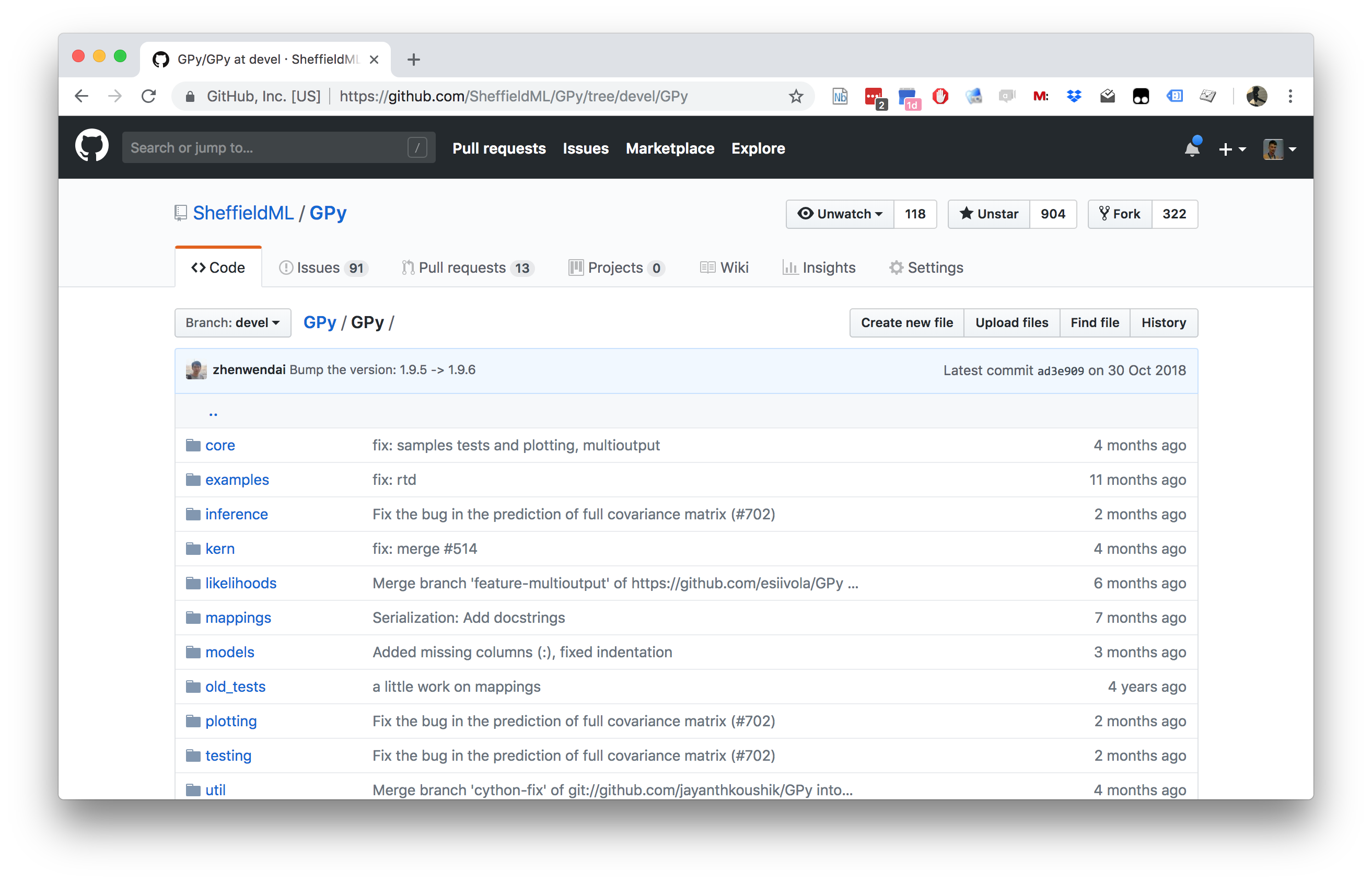
GPy: A Gaussian Process Framework in Python

• BSD Licensed software base.
• Wide availability of libraries, ‘modern’ scripting language.
• Allows us to set projects to undergraduates in Comp Sci that use GPs.
• Available through GitHub https://github.com/SheffieldML/GPy
• Reproducible Research with Jupyter Notebook.

Features

• Probabilistic-style programming (specify the model, not the algorithm).
• Non-Gaussian likelihoods.
• Multivariate outputs.
• Dimensionality reduction.
• Approximations for large data sets.

Selecting Data Dimensionality

• GP-LVM Provides probabilistic non-linear dimensionality reduction.
• How to select the dimensionality?
• Need to estimate marginal likelihood.
• In standard GP-LVM it increases with increasing \(q\).

Integrate Mapping Function and Latent Variables

Standard Variational Approach Fails

• Standard variational bound has the form: \[ \mathcal{L}= \left\langle\log p(\mathbf{ y}|\mathbf{Z})\right\rangle_{q(\mathbf{Z})} + \text{KL}\left( q(\mathbf{Z})\,\|\,p(\mathbf{Z}) \right) \]

Standard Variational Approach Fails

• Requires expectation of \(\log p(\mathbf{ y}|\mathbf{Z})\) under \(q(\mathbf{Z})\). \[ \begin{align} \log p(\mathbf{ y}|\mathbf{Z}) = & -\frac{1}{2}\mathbf{ y}^\top\left(\mathbf{K}_{\mathbf{ f}, \mathbf{ f}}+\sigma^2\mathbf{I}\right)^{-1}\mathbf{ y}\\ & -\frac{1}{2}\log \det{\mathbf{K}_{\mathbf{ f}, \mathbf{ f}}+\sigma^2 \mathbf{I}} -\frac{n}{2}\log 2\pi \end{align} \] \(\mathbf{K}_{\mathbf{ f}, \mathbf{ f}}\) is dependent on \(\mathbf{Z}\) and it appears in the inverse.

Variational Bayesian GP-LVM

• Consider collapsed variational bound, \[ p(\mathbf{ y})\geq \prod_{i=1}^nc_i \int \mathcal{N}\left(\mathbf{ y}|\left\langle\mathbf{ f}\right\rangle,\sigma^2\mathbf{I}\right)p(\mathbf{ u}) \text{d}\mathbf{ u} \] \[ p(\mathbf{ y}|\mathbf{Z})\geq \prod_{i=1}^nc_i \int \mathcal{N}\left(\mathbf{ y}|\left\langle\mathbf{ f}\right\rangle_{p(\mathbf{ f}|\mathbf{ u}, \mathbf{Z})},\sigma^2\mathbf{I}\right)p(\mathbf{ u}) \text{d}\mathbf{ u} \] \[ \int p(\mathbf{ y}|\mathbf{Z})p(\mathbf{Z}) \text{d}\mathbf{Z}\geq \int \prod_{i=1}^nc_i \mathcal{N}\left(\mathbf{ y}|\left\langle\mathbf{ f}\right\rangle_{p(\mathbf{ f}|\mathbf{ u}, \mathbf{Z})},\sigma^2\mathbf{I}\right) p(\mathbf{Z})\text{d}\mathbf{Z}p(\mathbf{ u}) \text{d}\mathbf{ u} \]

Variational Bayesian GP-LVM

• Apply variational lower bound to the inner integral. \[ \begin{align} \int \prod_{i=1}^nc_i \mathcal{N}\left(\mathbf{ y}|\left\langle\mathbf{ f}\right\rangle_{p(\mathbf{ f}|\mathbf{ u}, \mathbf{Z})},\sigma^2\mathbf{I}\right) p(\mathbf{Z})\text{d}\mathbf{Z}\geq & \left\langle\sum_{i=1}^n\log c_i\right\rangle_{q(\mathbf{Z})}\\ & +\left\langle\log\mathcal{N}\left(\mathbf{ y}|\left\langle\mathbf{ f}\right\rangle_{p(\mathbf{ f}|\mathbf{ u}, \mathbf{Z})},\sigma^2\mathbf{I}\right)\right\rangle_{q(\mathbf{Z})}\\& + \text{KL}\left( q(\mathbf{Z})\,\|\,p(\mathbf{Z}) \right) \end{align} \]
• Which is analytically tractable for Gaussian \(q(\mathbf{Z})\) and some covariance functions.

Required Expectations

• Need expectations under \(q(\mathbf{Z})\) of: \[ \log c_i = \frac{1}{2\sigma^2} \left[k_{i, i} - \mathbf{ k}_{i, \mathbf{ u}}^\top \mathbf{K}_{\mathbf{ u}, \mathbf{ u}}^{-1} \mathbf{ k}_{i, \mathbf{ u}}\right] \] and \[ \log \mathcal{N}\left(\mathbf{ y}|\left\langle\mathbf{ f}\right\rangle_{p(\mathbf{ f}|\mathbf{ u},\mathbf{Y})},\sigma^2\mathbf{I}\right) = -\frac{1}{2}\log 2\pi\sigma^2 - \frac{1}{2\sigma^2}\left(y_i - \mathbf{K}_{\mathbf{ f}, \mathbf{ u}}\mathbf{K}_{\mathbf{ u},\mathbf{ u}}^{-1}\mathbf{ u}\right)^2 \]

Required Expectations

• This requires the expectations \[ \left\langle\mathbf{K}_{\mathbf{ f},\mathbf{ u}}\right\rangle_{q(\mathbf{Z})} \] and \[ \left\langle\mathbf{K}_{\mathbf{ f},\mathbf{ u}}\mathbf{K}_{\mathbf{ u},\mathbf{ u}}^{-1}\mathbf{K}_{\mathbf{ u},\mathbf{ f}}\right\rangle_{q(\mathbf{Z})} \] which can be computed analytically for some covariance functions (Damianou et al., 2016) or through sampling (Damianou, 2015; Salimbeni and Deisenroth, 2017).

Manifold Relevance Determination

Modeling Multiple ‘Views’

• Single space to model correlations between two different data sources, e.g., images & text, image & pose.
• Shared latent spaces: Shon et al. (n.d.);Navaratnam et al. (2007);Ek et al. (2008b)
• Effective when the `views’ are correlated.
• But not all information is shared between both `views’.
• PCA applied to concatenated data vs CCA applied to data.

Shared-Private Factorization

• In real scenarios, the `views’ are neither fully independent, nor fully correlated.

• Shared models

  • either allow information relevant to a single view to be mixed in the shared signal,
  • or are unable to model such private information.

• Solution: Model shared and private information Virtanen et al. (n.d.),Ek et al. (2008a),Leen and Fyfe (2006),Klami and Kaski (n.d.),Klami and Kaski (2008),Tucker (1958)

• Probabilistic CCA is case when dimensionality of \(\mathbf{Z}\) matches \(\mathbf{Y}^{(i)}\) (cf Inter Battery Factor Analysis Tucker (1958)).

Manifold Relevance Determination

\def\layersep{2cm}
\begin{center}
  \begin{tikzpicture}[node distance=\layersep]

= [text width=4em, text centered] % Draw the input layer nodes / in {1,…,8} % This is the same as writing / in {1/1,2/2,3/3,4/4} (Y-) at (, 0) {\(y_\x\)};

% Draw the hidden layer nodes
\foreach \name / \x in {1,...,6}
    \path[xshift=1cm]
        node[latent] (X-\name) at (\x cm, \layersep) {$\latentScalar_\x$};

% Connect every node in the latent layer with every node in the
% data layer.
\foreach \source in {1,...,6}
    \foreach \dest in {1,...,8}
        \draw[->] (X-\source) -- (Y-\dest);



%  Annotate the layers
\node[annot,left of=X-1, node distance=1cm] (ls) {Latent space};
\node[annot,left of=Y-1, node distance=1cm] (ds) {Data space};

\end{tikzpicture} \end{center}

Shared GP-LVM

\def\layersep{2cm}
\begin{center}
  \begin{tikzpicture}[node distance=\layersep]

= [text width=4em, text centered] % Draw the input layer nodes / in {1,…,4} % This is the same as writing / in {1/1,2/2,3/3,4/4} (Y-) at (, 0) {\(y^{(1)}_\x\)};

\foreach \name / \x in {1,...,4}
% This is the same as writing \foreach \name / \x in {1/1,2/2,3/3,4/4}
    \node[obs] (Z-\name) at (\x+5, 0) {$\dataScalar^{(2)}_\x$};

% Draw the hidden layer nodes
\foreach \name / \x in {1,...,6}
    \path[xshift=2cm]
        node[latent] (X-\name) at (\x cm, \layersep) {$\latentScalar_\x$};

% Connect every node in the latent layer with every node in the
% data layer.
\foreach \source in {1,...,6}
    \foreach \dest in {1,...,4}
        \draw[->] (X-\source) -- (Y-\dest);

\foreach \source in {1,...,6}
    \foreach \dest in {1,...,4}
        \draw[->] (X-\source) -- (Z-\dest);


%  Annotate the layers
\node[annot,left of=X-1, node distance=1cm] (ls) {Latent space};
\node[annot,left of=Y-1, node distance=1cm] (ds) {Data space};

\end{tikzpicture} Separate ARD parameters for mappings to \(\mathbf{Y}^{(1)}\) and \(\mathbf{Y}^{(2)}\). \end{center}

Manifold Relevance Determination Results

Manifold Relevance Determination

Getting Started and Downloading Data

Bayesian GPLVM

Preoptimized Model

Multiview Learning: Manifold Relevance Determination

Interactive Demo: For Use Outside the Notepad

Observations

• We tend to obtain more “strange” outputs when sampling from latent space areas away from the training inputs.
• When sampling from the two dominant latent dimensions (the ones corresponding to large scales) we differentiate between all digits. Also note that projecting the latent space into the two dominant dimensions better separates the classes.
• When sampling from less dominant latent dimensions the outputs vary in a more subtle way.

Questions

• Can you see a difference in the ARD parameters to the non Bayesian GPLVM?
• How does the Bayesian GPLVM allow the ARD parameters of the RBF kernel magnify the two first dimensions?
• Is Bayesian GPLVM better in differentiating between different kinds of digits?
• Why does the starting noise variance have to be lower then the variance of the observed values?
• How come we use the lowest variance when using a linear kernel, but the highest lengtscale when using an RBF kernel?

Data for Blastocyst Development in Mice: Single Cell TaqMan Arrays

Principal Component Analysis

PCA Result

Bayesian GP-LVM