Week 8: Unsupervised Learning with Gaussian Processes

[Powerpoint][jupyter][google colab][reveal]

Abstract:

%pip install gpy

GPy: A Gaussian Process Framework in Python

Gaussian processes are a flexible tool for non-parametric analysis with uncertainty. The GPy software was started in Sheffield to provide a easy to use interface to GPs. One which allowed the user to focus on the modelling rather than the mathematics.

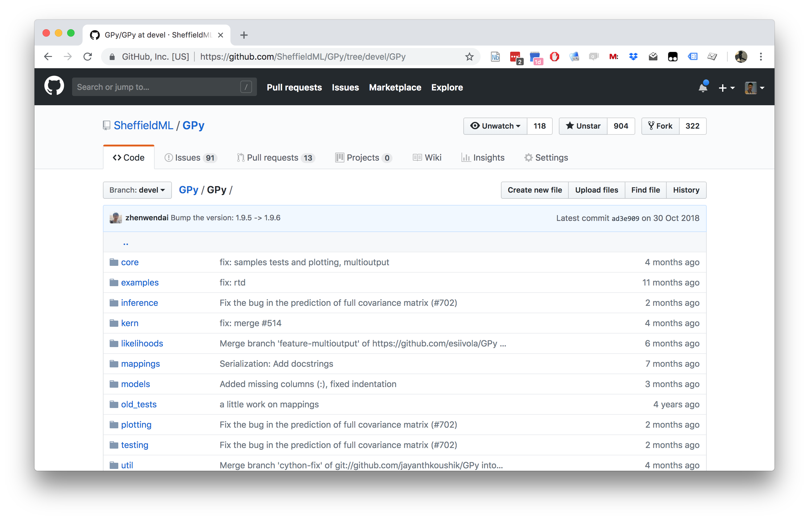
Figure: GPy is a BSD licensed software code base for implementing Gaussian process models in Python. It is designed for teaching and modelling. We welcome contributions which can be made through the GitHub repository https://github.com/SheffieldML/GPy

GPy is a BSD licensed software code base for implementing Gaussian process models in python. This allows GPs to be combined with a wide variety of software libraries.

The software itself is available on GitHub and the team welcomes contributions.

The aim for GPy is to be a probabilistic-style programming language, i.e., you specify the model rather than the algorithm. As well as a large range of covariance functions the software allows for non-Gaussian likelihoods, multivariate outputs, dimensionality reduction and approximations for larger data sets.

The documentation for GPy can be found here.

Probabilistic PCA

In 1997 Tipping and Bishop (Tipping and Bishop, 1999) and Roweis (Roweis, n.d.) independently revisited Hotelling’s model and considered the case where the noise variance was finite, but shared across all output dimensons. Their model can be thought of as a factor analysis where \[ \boldsymbol{\Sigma} = \sigma^2 \mathbf{I}. \] This leads to a marginal likelihood of the form \[ p(\mathbf{Y}|\mathbf{W}, \sigma^2) = \prod_{i=1}^n\mathcal{N}\left(\mathbf{ y}_{i, :}|\mathbf{0},\mathbf{W}\mathbf{W}^\top + \sigma^2 \mathbf{I}\right) \] where the limit of \(\sigma^2\rightarrow 0\) is not taken. This defines a proper probabilistic model. Tippping and Bishop then went on to prove that the maximum likelihood solution of this model with respect to \(\mathbf{W}\) is given by an eigenvalue problem. In the probabilistic PCA case the eigenvalues and eigenvectors are given as follows. \[ \mathbf{W}= \mathbf{U}\mathbf{L} \mathbf{R}^\top \] where \(\mathbf{U}\) is the eigenvectors of the empirical covariance matrix \[ \mathbf{S} = \sum_{i=1}^n(\mathbf{ y}_{i, :} - \boldsymbol{ \mu})(\mathbf{ y}_{i, :} - \boldsymbol{ \mu})^\top, \] which can be written \(\mathbf{S} = \frac{1}{n} \mathbf{Y}^\top\mathbf{Y}\) if the data is zero mean. The matrix \(\mathbf{L}\) is diagonal and is dependent on the eigenvalues of \(\mathbf{S}\), \(\boldsymbol{\Lambda}\). If the \(i\)th diagonal element of this matrix is given by \(\lambda_i\) then the corresponding element of \(\mathbf{L}\) is \[ \ell_i = \sqrt{\lambda_i - \sigma^2} \] where \(\sigma^2\) is the noise variance. Note that if \(\sigma^2\) is larger than any particular eigenvalue, then that eigenvalue (along with its corresponding eigenvector) is discarded from the solution.

Python Implementation of Probabilistic PCA

We will now implement this algorithm in python.

import numpy as np

# probabilistic PCA algorithm
def ppca(Y, q):
    # remove mean
    Y_cent = Y - Y.mean(0)

    # Comute covariance
    S = np.dot(Y_cent.T, Y_cent)/Y.shape[0]
    lambd, U = np.linalg.eig(S)

    # Choose number of eigenvectors
    sigma2 = np.sum(lambd[q:])/(Y.shape[1]-q)
    l = np.sqrt(lambd[:q]-sigma2)
    W = U[:, :q]*l[None, :]
    return W, sigma2

In practice we may not wish to compute the eigenvectors of the covariance matrix directly. This is because it requires us to estimate the covariance, which involves a sum of squares term, before estimating the eigenvectors. We can estimate the eigenvectors directly either through QR decomposition or singular value decomposition. We saw a similar issue arise when , where we also wished to avoid computation of \(\mathbf{Z}^\top\mathbf{Z}\) (or in the case of \(\boldsymbol{\Phi}^\top\boldsymbol{\Phi}\)).

Posterior for Principal Component Analysis

Under the latent variable model justification for principal component analysis, we are normally interested in inferring something about the latent variables given the data. This is the distribution, \[ p(\mathbf{ z}_{i, :} | \mathbf{ y}_{i, :}) \] for any given data point. Determining this density turns out to be very similar to the approach for determining the Bayesian posterior of \(\mathbf{ w}\) in Bayesian linear regression, only this time we place the prior density over \(\mathbf{ z}_{i, :}\) instead of \(\mathbf{ w}\). The posterior is proportional to the joint density as follows, \[ p(\mathbf{ z}_{i, :} | \mathbf{ y}_{i, :}) \propto p(\mathbf{ y}_{i, :}|\mathbf{W}, \mathbf{ z}_{i, :}, \sigma^2) p(\mathbf{ z}_{i, :}) \] And as in the Bayesian linear regression case we first consider the log posterior, \[ \log p(\mathbf{ z}_{i, :} | \mathbf{ y}_{i, :}) = \log p(\mathbf{ y}_{i, :}|\mathbf{W}, \mathbf{ z}_{i, :}, \sigma^2) + \log p(\mathbf{ z}_{i, :}) + \text{const} \] where the constant is not dependent on \(\mathbf{ z}\). As before we collect the quadratic terms in \(\mathbf{ z}_{i, :}\) and we assemble them into a Gaussian density over \(\mathbf{ z}\). \[ \log p(\mathbf{ z}_{i, :} | \mathbf{ y}_{i, :}) = -\frac{1}{2\sigma^2} (\mathbf{ y}_{i, :} - \mathbf{W}\mathbf{ z}_{i, :})^\top(\mathbf{ y}_{i, :} - \mathbf{W}\mathbf{ z}_{i, :}) - \frac{1}{2} \mathbf{ z}_{i, :}^\top \mathbf{ z}_{i, :} + \text{const} \]

Exercise 1

Multiply out the terms in the brackets. Then collect the quadratic term and the linear terms together. Show that the posterior has the form \[ \mathbf{ z}_{i, :} | \mathbf{W}\sim \mathcal{N}\left(\boldsymbol{ \mu}_x,\mathbf{C}_x\right) \] where \[ \mathbf{C}_x = \left(\sigma^{-2} \mathbf{W}^\top\mathbf{W}+ \mathbf{I}\right)^{-1} \] and \[ \boldsymbol{ \mu}_x = \mathbf{C}_x \sigma^{-2}\mathbf{W}^\top \mathbf{ y}_{i, :} \] Compare this to the posterior for the Bayesian linear regression from last week, do they have similar forms? What matches and what differs?

Python Implementation of the Posterior

Now let’s implement the system in code.

Exercise 2

Use the values for \(\mathbf{W}\) and \(\sigma^2\) you have computed, along with the data set \(\mathbf{Y}\) to compute the posterior density over \(\mathbf{Z}\). Write a function of the form

mu_x, C_x = posterior(Y, W, sigma2)

where mu_x and C_x are the posterior mean and posterior covariance for the given \(\mathbf{Y}\).

Don’t forget to subtract the mean of the data Y inside your function before computing the posterior: remember we assumed at the beginning of our analysis that the data had been centred (i.e. the mean was removed).

Numerically Stable and Efficient Version

Just as we saw for and computation of a matrix such as \(\mathbf{Y}^\top\mathbf{Y}\) (or its centred version) can be a bad idea in terms of loss of numerical accuracy. Fortunately, we can find the eigenvalues and eigenvectors of the matrix \(\mathbf{Y}^\top\mathbf{Y}\) without direct computation of the matrix. This can be done with the singular value decomposition. The singular value decompsition takes a matrix, \(\mathbf{Z}\) and represents it in the form, \[ \mathbf{Z} = \mathbf{U}\boldsymbol{\Lambda}\mathbf{V}^\top \] where \(\mathbf{U}\) is a matrix of orthogonal vectors in the columns, meaning \(\mathbf{U}^\top\mathbf{U} = \mathbf{I}\). It has the same number of rows and columns as \(\mathbf{Z}\). The matrices \(\mathbf{\Lambda}\) and \(\mathbf{V}\) are both square with dimensionality given by the number of columns of \(\mathbf{Z}\). The matrix \(\mathbf{\Lambda}\) is diagonal and \(\mathbf{V}\) is an orthogonal matrix so \(\mathbf{V}^\top\mathbf{V} = \mathbf{V}\mathbf{V}^\top = \mathbf{I}\). The eigenvalues of the matrix \(\mathbf{Y}^\top\mathbf{Y}\) are then given by the singular values of the matrix \(\mathbf{Y}^\top\) squared and the eigenvectors are given by \(\mathbf{U}\).

Solution for \(\mathbf{W}\)

Given the singular value decomposition of \(\mathbf{Y}\) then we have \[ \mathbf{W}= \mathbf{U}\mathbf{L}\mathbf{R}^\top \] where \(\mathbf{R}\) is an arbitrary rotation matrix. This implies that the posterior is given by \[ \mathbf{C}_x = \left[\sigma^{-2}\mathbf{R}\mathbf{L}^2\mathbf{R}^\top + \mathbf{I}\right]^{-1} \] because \(\mathbf{U}^\top \mathbf{U} = \mathbf{I}\). Since, by convention, we normally take \(\mathbf{R} = \mathbf{I}\) to ensure that the principal components are orthonormal we can write \[ \mathbf{C}_x = \left[\sigma^{-2}\mathbf{L}^2 + \mathbf{I}\right]^{-1} \] which implies that \(\mathbf{C}_x\) is actually diagonal with elements given by \[ c_i = \frac{\sigma^2}{\sigma^2 + \ell^2_i} \] and allows us to write \[ \boldsymbol{ \mu}_x = [\mathbf{L}^2 + \sigma^2 \mathbf{I}]^{-1} \mathbf{L} \mathbf{U}^\top \mathbf{ y}_{i, :} \] \[ \boldsymbol{ \mu}_x = \mathbf{D}\mathbf{U}^\top \mathbf{ y}_{i, :} \] where \(\mathbf{D}\) is a diagonal matrix with diagonal elements given by \(d_{i} = \frac{\ell_i}{\sigma^2 + \ell_i^2}\).

import scipy as sp
import numpy as np

# probabilistic PCA algorithm using SVD
def ppca(Y, q, center=True):
    """Probabilistic PCA through singular value decomposition"""
    # remove mean
    if center:
        Y_cent = Y - Y.mean(0)
    else:
        Y_cent = Y
        
    # Comute singluar values, discard 'R' as we will assume orthogonal
    U, sqlambd, _ = sp.linalg.svd(Y_cent.T,full_matrices=False)
    lambd = (sqlambd**2)/Y.shape[0]
    # Compute residual and extract eigenvectors
    sigma2 = np.sum(lambd[q:])/(Y.shape[1]-q)
    ell = np.sqrt(lambd[:q]-sigma2)
    return U[:, :q], ell, sigma2

def posterior(Y, U, ell, sigma2, center=True):
    """Posterior computation for the latent variables given the eigendecomposition."""
    if center:
        Y_cent = Y - Y.mean(0)
    else:
        Y_cent = Y
    C_x = np.diag(sigma2/(sigma2+ell**2))
    d = ell/(sigma2+ell**2)
    mu_x = np.dot(Y_cent, U)*d[None, :]
    return mu_x, C_x

Difficulty for Probabilistic Approaches

The challenge for composition of probabilistic models is that you need to propagate a probability densities through non linear mappings. This allows you to create broader classes of probability density. Unfortunately it renders the resulting densities intractable.

Figure: A two dimensional grid mapped into three dimensions to form a two dimensional manifold.

Figure: A one dimensional line mapped into two dimensions by two separate independent functions. Each point can be mapped exactly through the mappings.

Figure: A Gaussian density over the input of a non linear function leads to a very non Gaussian output. Here the output is multimodal.

Getting Started and Downloading Data

import numpy as np
import GPy
import string

The following code is for plotting and to prepare the bigger models for later useage. If you are interested, you can have a look, but this is not essential.

For this lab, we’ll use a data set containing all handwritten digits from \(0 \cdots 9\) handwritten, provided by de Campos et al. (2009). We will only use some of the digits for the demonstrations in this lab class, but you can edit the code below to select different subsets of the digit data as you wish.

which = [0,1,2,6,7,9] # which digits to work on
data = pods.datasets.decampos_digits(which_digits=which)
Y = data['Y']
labels = data['str_lbls']

You can try to plot some of the digits using plt.matshow (the digit images have size 16x16).

Principal Component Analysis

Principal component analysis (PCA) finds a rotation of the observed outputs, such that the rotated principal component (PC) space maximizes the variance of the data observed, sorted from most to least important (most to least variable in the corresponding PC).

In order to apply PCA in an easy way, we have included a PCA module in pca.py. You can import the module by import <path.to.pca> (without the ending .py!). To run PCA on the digits we have to reshape (Hint: np.reshape ) digits .

• What is the right shape \(n\times p\) to use?

We will call the reshaped observed outputs \(\mathbf{Y}\) in the following.

Yn = Y#Y-Y.mean()

Now let’s run PCA on the reshaped dataset \(\mathbf{Y}\):

from GPy.util import pca
p = pca.pca(Y) # create PCA class with digits dataset

The resulting plot will show the lower dimensional representation of the digits in 2 dimensions.

Gaussian Process Latent Variable Model

The Gaussian Process Latent Variable Model (GP-LVM) (Lawrence, 2005) embeds PCA into a Gaussian process framework, where the latent inputs \(\mathbf{Z}\) are learnt as hyperparameters and the mapping variables \(\mathbf{W}\) are integrated out. The advantage of this interpretation is it allows PCA to be generalized in a non linear way by replacing the resulting linear covariance witha non linear covariance. But first, let’s see how GPLVM is equivalent to PCA using an automatic relevance determination (ARD, see e.g. Bishop (2006)) linear kernel:

input_dim = 4 # How many latent dimensions to use
kernel = GPy.kern.Linear(input_dim, ARD=True) # ARD kernel
m = GPy.models.GPLVM(Yn, input_dim=input_dim, kernel=kernel)

m.optimize(messages=1, max_iters=1000) # optimize for 1000 iterations

As you can see the solution with a linear kernel is the same as the PCA solution with the exception of rotational changes and axis flips.

For the sake of time, the solution you see was only running for 1000 iterations, thus it might not be converged fully yet. The GP-LVM proceeds by iterative optimization of the inputs to the covariance. As we saw in the lecture earlier, for the linear covariance, these latent points can be optimized with an eigenvalue problem, but generally, for non-linear covariance functions, we are obliged to use gradient based optimization.

CMU Mocap Database

Motion capture data from the CMU motion capture data base (CMU Motion Capture Lab, 2003).

import pods

You can download any subject and motion from the data set. Here we will download motion 01 from subject 35.

subject='35' 
motion=['01']

data = pods.datasets.cmu_mocap(subject, motion)

The data dictionary contains the keys ‘Y’ and ‘skel’, which represent the data and the skeleton..

data['Y'].shape

The data was used in the hierarchical GP-LVM paper (Lawrence and Moore, 2007) in an experiment that was also recreated in the Deep Gaussian process paper (Damianou and Lawrence, 2013).

print(data['citation'])

And extra information about the data is included, as standard, under the keys info and details.

print(data['info'])
print()
print(data['details'])

CMU Motion Capture GP-LVM

The original data has the figure moving across the floor during the motion capture sequence. We can make the figure walk ‘in place’, by setting the x, y, z positions of the root node to zero. This makes it easier to visualize the result.

# Make figure move in place.
data['Y'][:, 0:3] = 0.0

We can also remove the mean of the data.

Y = data['Y']

Now we create the GP-LVM model.

import GPy

model = GPy.models.GPLVM(Y, 2, normalizer=True)

Now we optimize the model.

model.optimize(messages=True, max_f_eval=10000)

Figure: Gaussian process latent variable model visualisation of CMU motion capture data set.

Example: Latent Doodle Space

Figure: The latent doodle space idea of Baxter and Anjyo (2006) manages to build a smooth mapping across very sparse data.

Generalization with much less Data than Dimensions

• Powerful uncertainly handling of GPs leads to surprising properties.

• Non-linear models can be used where there are fewer data points than dimensions without overfitting.

Example: Continuous Character Control

• Graph diffusion prior for enforcing connectivity between motions. \[\log p(\mathbf{X}) = w_c \sum_{i,j} \log K_{ij}^d\] with the graph diffusion kernel \(\mathbf{K}^d\) obtain from \[K_{ij}^d = \exp(\beta \mathbf{H}) \qquad \text{with} \qquad \mathbf{H} = -\mathbf{T}^{-1/2} \mathbf{L} \mathbf{T}^{-1/2}\] the graph Laplacian, and \(\mathbf{T}\) is a diagonal matrix with \(T_{ii} = \sum_j w(\mathbf{ x}_i, \mathbf{ x}_j)\), \[L_{ij} = \begin{cases} \sum_k w(\mathbf{ x}_i,\mathbf{ x}_k) & \text{if $i=j$} \\ -w(\mathbf{ x}_i,\mathbf{ x}_j) &\text{otherwise.} \end{cases}\] and \(w(\mathbf{ x}_i,\mathbf{ x}_j) = || \mathbf{ x}_i - \mathbf{ x}_j||^{-p}\) measures similarity.

Character Control: Results

Figure: Character control in the latent space described the the GP-LVM Levine et al. (2012).

Data for Blastocyst Development in Mice: Single Cell TaqMan Arrays

Now we analyze some single cell data from Guo et al. (2010). Tey performed qPCR TaqMan array on single cells from the developing blastocyst in mouse. The data is taken from the early stages of development when the Blastocyst is forming. At the 32 cell stage the data is already separated into the trophectoderm (TE) which goes onto form the placenta and the inner cellular mass (ICM). The ICM further differentiates into the epiblast (EPI)—which gives rise to the endoderm, mesoderm and ectoderm—and the primitive endoderm (PE) which develops into the amniotic sack. Guo et al. (2010) selected 48 genes for expression measurement. They labelled the resulting cells and their labels are included as an aide to visualization.

They first visualized their data using principal component analysis. In the first two principal components this fails to separate the domains. This is perhaps because the principal components are dominated by the variation in the 64 cell systems. This in turn may be because there are more cells from the data set in that regime, and may be because the natural variation is greater. We first recreate their visualization using principal component analysis.

In this notebook we will perform PCA on the original data, showing that the different regimes do not separate.

Next we load in the data. We’ve provided a convenience function for loading in the data with pods. It is loaded in as a pandas DataFrame. This allows us to summarize it with the describe attribute.

import pods

data = pods.datasets.singlecell()
Y = data['Y']
Y.describe

Principal Component Analysis

Now we follow Guo et al. (2010) in performing PCA on the data. Rather than calling a ‘PCA routine’, here we break the algorithm down into its steps: compute the data covariance, compute the eigenvalues and eigenvectors and sort according to magnitude of eigenvalue. Because we want to visualize the data, we’ve chose to compute the eigenvectors of the inner product matrix rather than the covariance matrix. This allows us to plot the eigenvalues directly. However, this is less efficient (in this case because the number of genes is smaller than the number of data) than computing the eigendecomposition of the covariance matrix.

import numpy as np

# obtain a centred version of data.
centredY = Y - Y.mean()
# compute inner product matrix
C = np.dot(centredY,centredY.T)
# perform eigendecomposition
V, U = np.linalg.eig(C)
# sort eigenvalues and vectors according to size
ind = V.argsort()
ev = V[ind[::-1]]
U = U[:, ind[::-1]]

To visualize the result, we now construct a simple helper function. This will ensure that the plots have the same legends as the GP-LVM plots we use below.

PCA Result

Now, using the helper function we can plot the results with appropriate labels.

Figure: First two principal compoents of the Guo et al. (2010) blastocyst development data.

GP-LVM on the Data

Work done as a collaboration between Max Zwiessele, Oliver Stegle and Neil D. Lawrence.

Then, we follow Buettner and Theis (2012) in applying the GP-LVM to the data. There is a slight pathology in the result, one which they fixed by using priors that were dependent on the developmental stage. We then show how the Bayesian GP-LVM doesn’t exhibit those pathologies and gives a nice results that seems to show the lineage of the cells.

They used modified prior to ensure that small differences between cells at the same differential stage were preserved. Here we apply a standard GP-LVM (no modified prior) to the data.

import GPy

kernel = GPy.kern.RBF(2)+GPy.kern.Bias(2)
model = GPy.models.GPLVM(Y.values, 2, kernel=kernel)
model.optimize(messages=True)

Figure: Visualisation of the Guo et al. (2010) blastocyst development data with the GP-LVM.

Figure: The ARD parameters of the GP-LVM for the Guo et al. (2010) blastocyst development data.

Blastocyst Data: Isomap

Isomap first builds a neighbourhood graph, and then uses distances along this graph to approximate the geodesic distance between points. These distances are then visualized by performing classical multidimensional scaling (which involves computing the eigendecomposition of the centred distance matrix). As the neighborhood size is increased to match the data, principal component analysis is recovered (or strictly speaking, principal coordinate analysis). The fewer the neighbors, the more ‘non-linear’ the isomap embeddings are.

import sklearn.manifold

n_neighbors = 10
model = sklearn.manifold.Isomap(n_neighbors=n_neighbors, n_components=2)
X = model.fit_transform(Y)

Figure: Visualisation of the Guo et al. (2010) blastocyst development data with Isomap.

Blastocyst Data: Locally Linear Embedding

Next we try locally linear embedding. In locally linear embedding a neighborhood is also computed. Each point is then reconstructed by it’s neighbors using a linear weighting. This implies a locally linear patch is being fitted to the data in that region. These patches are assimilated into a large \(n\times n\) matrix and a lower dimensional data set which reflects the same relationships is then sought. Quite a large number of neighbours needs to be selected for the data to not collapse in on itself. When a large number of neighbours is selected the embedding is more linear and begins to look like PCA. However, the algorithm does not converge to PCA in the limit as the number of neighbors approaches \(n\).

import sklearn.manifold

n_neighbors = 50
model = sklearn.manifold.LocallyLinearEmbedding(n_neighbors=n_neighbors, n_components=2)
X = model.fit_transform(Y)

Figure: Visualisation of the Guo et al. (2010) blastocyst development data with a locally linear embedding.

Thanks!

For more information on these subjects and more you might want to check the following resources.

• twitter: @lawrennd
• podcast: The Talking Machines
• newspaper: Guardian Profile Page
• blog: http://inverseprobability.com

References