Week 4: Optimizing Parameters

[Powerpoint][jupyter][google colab][reveal]

Abstract:

In this session we introduce the process of optimization of the hyper parameters of the Gaussian process covariance function.

%pip install gpy

GPy: A Gaussian Process Framework in Python

Gaussian processes are a flexible tool for non-parametric analysis with uncertainty. The GPy software was started in Sheffield to provide a easy to use interface to GPs. One which allowed the user to focus on the modelling rather than the mathematics.

Figure: GPy is a BSD licensed software code base for implementing Gaussian process models in Python. It is designed for teaching and modelling. We welcome contributions which can be made through the GitHub repository https://github.com/SheffieldML/GPy

GPy is a BSD licensed software code base for implementing Gaussian process models in python. This allows GPs to be combined with a wide variety of software libraries.

The software itself is available on GitHub and the team welcomes contributions.

The aim for GPy is to be a probabilistic-style programming language, i.e., you specify the model rather than the algorithm. As well as a large range of covariance functions the software allows for non-Gaussian likelihoods, multivariate outputs, dimensionality reduction and approximations for larger data sets.

The documentation for GPy can be found here.

Improving the Numerics

In practice we shouldn’t be using matrix inverse directly to solve the GP system. One more stable way is to compute the Cholesky decomposition of the kernel matrix. The log determinant of the covariance can also be derived from the Cholesky decomposition.

import mlai

from mlai import update_inverse

GP.update_inverse = update_inverse

Capacity Control

Gaussian processes are sometimes seen as part of a wider family of methods known as kernel methods. Kernel methods are also based around covariance functions, but in the field they are known as Mercer kernels. Mercer kernels have interpretations as inner products in potentially infinite dimensional Hilbert spaces. This interpretation arises because, if we take \(\alpha=1\), then the kernel can be expressed as \[ \mathbf{K}= \boldsymbol{ \Phi}\boldsymbol{ \Phi}^\top \] which imples the elements of the kernel are given by, \[ k(\mathbf{ x}, \mathbf{ x}^\prime) = \boldsymbol{ \phi}(\mathbf{ x})^\top \boldsymbol{ \phi}(\mathbf{ x}^\prime). \] So we see that the kernel function is developed from an inner product between the basis functions. Mercer’s theorem tells us that any valid positive definite function can be expressed as this inner product but with the caveat that the inner product could be infinite length. This idea has been used quite widely to kernelize algorithms that depend on inner products. The kernel functions are equivalent to covariance functions and they are parameterized accordingly. In the kernel modeling community it is generally accepted that kernel parameter estimation is a difficult problem and the normal solution is to cross validate to obtain parameters. This can cause difficulties when a large number of kernel parameters need to be estimated. In Gaussian process modelling kernel parameter estimation (in the simplest case proceeds) by maximum likelihood. This involves taking gradients of the likelihood with respect to the parameters of the covariance function.

Gradients of the Likelihood

The easiest conceptual way to obtain the gradients is a two step process. The first step involves taking the gradient of the likelihood with respect to the covariance function, the second step involves considering the gradient of the covariance function with respect to its parameters.

Overall Process Scale

In general we won’t be able to find parameters of the covariance function through fixed point equations, we will need to do gradient based optimization.

Capacity Control and Data Fit

The objective function can be decomposed into two terms, a capacity control term, and a data fit term. The capacity control term is the log determinant of the covariance. The data fit term is the matrix inner product between the data and the inverse covariance.

Learning Covariance Parameters

Can we determine covariance parameters from the data?

\[ \mathcal{N}\left(\mathbf{ y}|\mathbf{0},\mathbf{K}\right)=\frac{1}{(2\pi)^\frac{n}{2}{\det{\mathbf{K}}^{\frac{1}{2}}}}{\exp\left(-\frac{\mathbf{ y}^{\top}\mathbf{K}^{-1}\mathbf{ y}}{2}\right)} \]

\[ \begin{aligned} \mathcal{N}\left(\mathbf{ y}|\mathbf{0},\mathbf{K}\right)=\frac{1}{(2\pi)^\frac{n}{2}\color{blue}{\det{\mathbf{K}}^{\frac{1}{2}}}}\color{red}{\exp\left(-\frac{\mathbf{ y}^{\top}\mathbf{K}^{-1}\mathbf{ y}}{2}\right)} \end{aligned} \]

\[ \begin{aligned} \log \mathcal{N}\left(\mathbf{ y}|\mathbf{0},\mathbf{K}\right)=&\color{blue}{-\frac{1}{2}\log\det{\mathbf{K}}}\color{red}{-\frac{\mathbf{ y}^{\top}\mathbf{K}^{-1}\mathbf{ y}}{2}} \\ &-\frac{n}{2}\log2\pi \end{aligned} \]

\[ E(\boldsymbol{ \theta}) = \color{blue}{\frac{1}{2}\log\det{\mathbf{K}}} + \color{red}{\frac{\mathbf{ y}^{\top}\mathbf{K}^{-1}\mathbf{ y}}{2}} \]

Capacity Control through the Determinant

The parameters are inside the covariance function (matrix). \[k_{i, j} = k(\mathbf{ x}_i, \mathbf{ x}_j; \boldsymbol{ \theta})\]

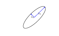
\[\mathbf{K}= \mathbf{R}\boldsymbol{ \Lambda}^2 \mathbf{R}^\top\]

\(\boldsymbol{ \Lambda}\) represents distance on axes. \(\mathbf{R}\) gives rotation.

• \(\boldsymbol{ \Lambda}\) is diagonal, \(\mathbf{R}^\top\mathbf{R}= \mathbf{I}\).
• Useful representation since \(\det{\mathbf{K}} = \det{\boldsymbol{ \Lambda}^2} = \det{\boldsymbol{ \Lambda}}^2\).

Figure: The determinant of the covariance is dependent only on the eigenvalues. It represents the ‘footprint’ of the Gaussian.

Quadratic Data Fit

Figure: The data fit term of the Gaussian process is a quadratic loss centered around zero. This has eliptical contours, the principal axes of which are given by the covariance matrix.

Data Fit Term

Figure: Variation in the data fit term, the capacity term and the negative log likelihood for different lengthscales.

Gene Expression Example

We now consider an example in gene expression. Gene expression is the measurement of mRNA levels expressed in cells. These mRNA levels show which genes are ‘switched on’ and producing data. In the example we will use a Gaussian process to determine whether a given gene is active, or we are merely observing a noise response.

Della Gatta Gene Data

• Given given expression levels in the form of a time series from Della Gatta et al. (2008).

import numpy as np
import pods

data = pods.datasets.della_gatta_TRP63_gene_expression(data_set='della_gatta',gene_number=937)

x = data['X']
y = data['Y']

offset = y.mean()
scale = np.sqrt(y.var())

Figure: Gene expression levels over time for a gene from data provided by Della Gatta et al. (2008). We would like to understand whether there is signal in the data, or we are only observing noise.

• Want to detect if a gene is expressed or not, fit a GP to each gene Kalaitzis and Lawrence (2011).

Figure: The example is taken from the paper “A Simple Approach to Ranking Differentially Expressed Gene Expression Time Courses through Gaussian Process Regression.” Kalaitzis and Lawrence (2011).

Our first objective will be to perform a Gaussian process fit to the data, we’ll do this using the GPy software.

import GPy

m_full = GPy.models.GPRegression(x,yhat)
m_full.kern.lengthscale=50
_ = m_full.optimize() # Optimize parameters of covariance function

Initialize the length scale parameter (which here actually represents a time scale of the covariance function) to a reasonable value. Default would be 1, but here we set it to 50 minutes, given points are arriving across zero to 250 minutes.

xt = np.linspace(-20,260,200)[:,np.newaxis]
yt_mean, yt_var = m_full.predict(xt)
yt_sd=np.sqrt(yt_var)

Now we plot the results using the helper function in mlai.plot.

Figure: Result of the fit of the Gaussian process model with the time scale parameter initialized to 50 minutes.

Now we try a model initialized with a longer length scale.

m_full2 = GPy.models.GPRegression(x,yhat)
m_full2.kern.lengthscale=2000
_ = m_full2.optimize() # Optimize parameters of covariance function

Figure: Result of the fit of the Gaussian process model with the time scale parameter initialized to 2000 minutes.

Now we try a model initialized with a lower noise.

m_full3 = GPy.models.GPRegression(x,yhat)
m_full3.kern.lengthscale=20
m_full3.likelihood.variance=0.001
_ = m_full3.optimize() # Optimize parameters of covariance function

Figure: Result of the fit of the Gaussian process model with the noise initialized low (standard deviation 0.1) and the time scale parameter initialized to 20 minutes.

Figure:

Thanks!

For more information on these subjects and more you might want to check the following resources.

• twitter: @lawrennd
• podcast: The Talking Machines
• newspaper: Guardian Profile Page
• blog: http://inverseprobability.com

References