Optimizing Parameters

GPy: A Gaussian Process Framework in Python

GPy: A Gaussian Process Framework in Python

• BSD Licensed software base.
• Wide availability of libraries, ‘modern’ scripting language.
• Allows us to set projects to undergraduates in Comp Sci that use GPs.
• Available through GitHub https://github.com/SheffieldML/GPy
• Reproducible Research with Jupyter Notebook.

Features

• Probabilistic-style programming (specify the model, not the algorithm).
• Non-Gaussian likelihoods.
• Multivariate outputs.
• Dimensionality reduction.
• Approximations for large data sets.

Improving the Numerics

In practice we shouldn’t be using matrix inverse directly to solve the GP system. One more stable way is to compute the Cholesky decomposition of the kernel matrix. The log determinant of the covariance can also be derived from the Cholesky decomposition.

Capacity Control

Gradients of the Likelihood

Overall Process Scale

Capacity Control and Data Fit

Learning Covariance Parameters

Can we determine covariance parameters from the data?

\[ \mathcal{N}\left(\mathbf{ y}|\mathbf{0},\mathbf{K}\right)=\frac{1}{(2\pi)^\frac{n}{2}{\det{\mathbf{K}}^{\frac{1}{2}}}}{\exp\left(-\frac{\mathbf{ y}^{\top}\mathbf{K}^{-1}\mathbf{ y}}{2}\right)} \]

\[ \begin{aligned} \mathcal{N}\left(\mathbf{ y}|\mathbf{0},\mathbf{K}\right)=\frac{1}{(2\pi)^\frac{n}{2}\color{yellow}{\det{\mathbf{K}}^{\frac{1}{2}}}}\color{cyan}{\exp\left(-\frac{\mathbf{ y}^{\top}\mathbf{K}^{-1}\mathbf{ y}}{2}\right)} \end{aligned} \]

\[ \begin{aligned} \log \mathcal{N}\left(\mathbf{ y}|\mathbf{0},\mathbf{K}\right)=&\color{yellow}{-\frac{1}{2}\log\det{\mathbf{K}}}\color{cyan}{-\frac{\mathbf{ y}^{\top}\mathbf{K}^{-1}\mathbf{ y}}{2}} \\ &-\frac{n}{2}\log2\pi \end{aligned} \]

\[ E(\boldsymbol{ \theta}) = \color{yellow}{\frac{1}{2}\log\det{\mathbf{K}}} + \color{cyan}{\frac{\mathbf{ y}^{\top}\mathbf{K}^{-1}\mathbf{ y}}{2}} \]

Capacity Control through the Determinant

The parameters are inside the covariance function (matrix). \[k_{i, j} = k(\mathbf{ x}_i, \mathbf{ x}_j; \boldsymbol{ \theta})\]

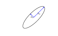
Eigendecomposition of Covariance

\[\mathbf{K}= \mathbf{R}\boldsymbol{ \Lambda}^2 \mathbf{R}^\top\]

\(\boldsymbol{ \Lambda}\) represents distance on axes. \(\mathbf{R}\) gives rotation.

Eigendecomposition of Covariance

• \(\boldsymbol{ \Lambda}\) is diagonal, \(\mathbf{R}^\top\mathbf{R}= \mathbf{I}\).
• Useful representation since \(\det{\mathbf{K}} = \det{\boldsymbol{ \Lambda}^2} = \det{\boldsymbol{ \Lambda}}^2\).

Capacity control: \(\color{yellow}{\log \det{\mathbf{K}}}\)

❮ ❯

Quadratic Data Fit

Data Fit: \(\color{cyan}{\frac{\mathbf{ y}^\top\mathbf{K}^{-1}\mathbf{ y}}{2}}\)

❮ ❯

\[E(\boldsymbol{ \theta}) = \color{yellow}{\frac{1}{2}\log\det{\mathbf{K}}}+\color{cyan}{\frac{\mathbf{ y}^{\top}\mathbf{K}^{-1}\mathbf{ y}}{2}}\]

Data Fit Term

❮ ❯

Della Gatta Gene Data

• Given given expression levels in the form of a time series from Della Gatta et al. (2008).

Della Gatta Gene Data

Gene Expression Example

• Want to detect if a gene is expressed or not, fit a GP to each gene Kalaitzis and Lawrence (2011).

TP53 Gene Data GP

TP53 Gene Data GP

TP53 Gene Data GP

Multiple Optima