Week 3: Covariance Functions and Hyperparameter Optimization

[Powerpoint][jupyter][google colab][reveal]

Neil D. Lawrence

Abstract:

In this talk we review covariance functions and optimization of the GP log likelihoood.

%pip install gpy

GPy: A Gaussian Process Framework in Python

Gaussian processes are a flexible tool for non-parametric analysis with uncertainty. The GPy software was started in Sheffield to provide a easy to use interface to GPs. One which allowed the user to focus on the modelling rather than the mathematics.

Figure: GPy is a BSD licensed software code base for implementing Gaussian process models in Python. It is designed for teaching and modelling. We welcome contributions which can be made through the GitHub repository https://github.com/SheffieldML/GPy

GPy is a BSD licensed software code base for implementing Gaussian process models in python. This allows GPs to be combined with a wide variety of software libraries.

The software itself is available on GitHub and the team welcomes contributions.

The aim for GPy is to be a probabilistic-style programming language, i.e., you specify the model rather than the algorithm. As well as a large range of covariance functions the software allows for non-Gaussian likelihoods, multivariate outputs, dimensionality reduction and approximations for larger data sets.

The documentation for GPy can be found here.

The Importance of the Covariance Function

The covariance function encapsulates our assumptions about the data. The equations for the distribution of the prediction function, given the training observations, are highly sensitive to the covariation between the test locations and the training locations as expressed by the matrix \(\mathbf{K}_*\). We defined a matrix \(\mathbf{A}\) which allowed us to express our conditional mean in the form, \[ \boldsymbol{ \mu}_f= \mathbf{A}^\top \mathbf{ y}, \] where \(\mathbf{ y}\) were our training observations. In other words our mean predictions are always a linear weighted combination of our training data. The weights are given by computing the covariation between the training and the test data (\(\mathbf{K}_*\)) and scaling it by the inverse covariance of the training data observations, \(\left[\mathbf{K}+ \sigma^2 \mathbf{I}\right]^{-1}\). This inverse is the main computational object that needs to be resolved for a Gaussian process. It has a computational burden which is \(O(n^3)\) and a storage burden which is \(O(n^2)\). This makes working with Gaussian processes computationally intensive for the situation where \(n>10,000\).

Figure: Introduction to Gaussian processes given by Neil Lawrence at the 2014 Gaussian process Winter School at the University of Sheffield.

Improving the Numerics

In practice we shouldn’t be using matrix inverse directly to solve the GP system. One more stable way is to compute the Cholesky decomposition of the kernel matrix. The log determinant of the covariance can also be derived from the Cholesky decomposition.

import mlai

from mlai import update_inverse

GP.update_inverse = update_inverse

Capacity Control

Gaussian processes are sometimes seen as part of a wider family of methods known as kernel methods. Kernel methods are also based around covariance functions, but in the field they are known as Mercer kernels. Mercer kernels have interpretations as inner products in potentially infinite dimensional Hilbert spaces. This interpretation arises because, if we take \(\alpha=1\), then the kernel can be expressed as \[ \mathbf{K}= \boldsymbol{ \Phi}\boldsymbol{ \Phi}^\top \] which imples the elements of the kernel are given by, \[ k(\mathbf{ x}, \mathbf{ x}^\prime) = \boldsymbol{ \phi}(\mathbf{ x})^\top \boldsymbol{ \phi}(\mathbf{ x}^\prime). \] So we see that the kernel function is developed from an inner product between the basis functions. Mercer’s theorem tells us that any valid positive definite function can be expressed as this inner product but with the caveat that the inner product could be infinite length. This idea has been used quite widely to kernelize algorithms that depend on inner products. The kernel functions are equivalent to covariance functions and they are parameterized accordingly. In the kernel modeling community it is generally accepted that kernel parameter estimation is a difficult problem and the normal solution is to cross validate to obtain parameters. This can cause difficulties when a large number of kernel parameters need to be estimated. In Gaussian process modelling kernel parameter estimation (in the simplest case proceeds) by maximum likelihood. This involves taking gradients of the likelihood with respect to the parameters of the covariance function.

Gradients of the Likelihood

The easiest conceptual way to obtain the gradients is a two step process. The first step involves taking the gradient of the likelihood with respect to the covariance function, the second step involves considering the gradient of the covariance function with respect to its parameters.

Overall Process Scale

In general we won’t be able to find parameters of the covariance function through fixed point equations, we will need to do gradient based optimization.

Capacity Control and Data Fit

The objective function can be decomposed into two terms, a capacity control term, and a data fit term. The capacity control term is the log determinant of the covariance. The data fit term is the matrix inner product between the data and the inverse covariance.

Learning Covariance Parameters

Can we determine covariance parameters from the data?

\[ \mathcal{N}\left(\mathbf{ y}|\mathbf{0},\mathbf{K}\right)=\frac{1}{(2\pi)^\frac{n}{2}{\det{\mathbf{K}}^{\frac{1}{2}}}}{\exp\left(-\frac{\mathbf{ y}^{\top}\mathbf{K}^{-1}\mathbf{ y}}{2}\right)} \]

\[ \begin{aligned} \mathcal{N}\left(\mathbf{ y}|\mathbf{0},\mathbf{K}\right)=\frac{1}{(2\pi)^\frac{n}{2}\color{blue}{\det{\mathbf{K}}^{\frac{1}{2}}}}\color{red}{\exp\left(-\frac{\mathbf{ y}^{\top}\mathbf{K}^{-1}\mathbf{ y}}{2}\right)} \end{aligned} \]

\[ \begin{aligned} \log \mathcal{N}\left(\mathbf{ y}|\mathbf{0},\mathbf{K}\right)=&\color{blue}{-\frac{1}{2}\log\det{\mathbf{K}}}\color{red}{-\frac{\mathbf{ y}^{\top}\mathbf{K}^{-1}\mathbf{ y}}{2}} \\ &-\frac{n}{2}\log2\pi \end{aligned} \]

\[ E(\boldsymbol{ \theta}) = \color{blue}{\frac{1}{2}\log\det{\mathbf{K}}} + \color{red}{\frac{\mathbf{ y}^{\top}\mathbf{K}^{-1}\mathbf{ y}}{2}} \]

Capacity Control through the Determinant

The parameters are inside the covariance function (matrix). \[k_{i, j} = k(\mathbf{ x}_i, \mathbf{ x}_j; \boldsymbol{ \theta})\]

\[\mathbf{K}= \mathbf{R}\boldsymbol{ \Lambda}^2 \mathbf{R}^\top\]

\(\boldsymbol{ \Lambda}\) represents distance on axes. \(\mathbf{R}\) gives rotation.

• \(\boldsymbol{ \Lambda}\) is diagonal, \(\mathbf{R}^\top\mathbf{R}= \mathbf{I}\).
• Useful representation since \(\det{\mathbf{K}} = \det{\boldsymbol{ \Lambda}^2} = \det{\boldsymbol{ \Lambda}}^2\).

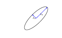
Figure: The determinant of the covariance is dependent only on the eigenvalues. It represents the ‘footprint’ of the Gaussian.

Quadratic Data Fit

Figure: The data fit term of the Gaussian process is a quadratic loss centered around zero. This has eliptical contours, the principal axes of which are given by the covariance matrix.

Data Fit Term

Figure: Variation in the data fit term, the capacity term and the negative log likelihood for different lengthscales.

Exponentiated Quadratic Covariance

The exponentiated quadratic covariance, also known as the Gaussian covariance or the RBF covariance and the squared exponential. Covariance between two points is related to the negative exponential of the squared distnace between those points. This covariance function can be derived in a few different ways: as the infinite limit of a radial basis function neural network, as diffusion in the heat equation, as a Gaussian filter in Fourier space or as the composition as a series of linear filters applied to a base function.

The covariance takes the following form, \[ k(\mathbf{ x}, \mathbf{ x}^\prime) = \alpha \exp\left(-\frac{\left\Vert \mathbf{ x}-\mathbf{ x}^\prime \right\Vert_2^2}{2\ell^2}\right) \] where \(\ell\) is the length scale or time scale of the process and \(\alpha\) represents the overall process variance.

Figure: The exponentiated quadratic covariance function.

Where Did This Covariance Matrix Come From?

\[ k(\mathbf{ x}, \mathbf{ x}^\prime) = \alpha \exp\left(-\frac{\left\Vert \mathbf{ x}- \mathbf{ x}^\prime\right\Vert^2_2}{2\ell^2}\right)\]

Figure: Entrywise fill in of the covariance matrix from the covariance function.

Figure: Entrywise fill in of the covariance matrix from the covariance function.

Figure: Entrywise fill in of the covariance matrix from the covariance function.

Brownian Covariance

import mlai

from mlai import brownian_cov

Brownian motion is also a Gaussian process. It follows a Gaussian random walk, with diffusion occuring at each time point driven by a Gaussian input. This implies it is both Markov and Gaussian. The covariance function for Brownian motion has the form \[ k(t, t^\prime)=\alpha \min(t, t^\prime) \]

Figure: Brownian motion covariance function.

Where did this covariance matrix come from?

Markov Process

Visualization of inverse covariance (precision).

• Precision matrix is sparse: only neighbours in matrix are non-zero.

• This reflects conditional independencies in data.

• In this case Markov structure.

Where did this covariance matrix come from?

Exponentiated Quadratic

Visualization of inverse covariance (precision).

Covariance Functions

Markov Process

Visualization of inverse covariance (precision).

Exponential Covariance

The expontential covariance, in one dimension this is also known as the Ornstein Uhlenbeck covariance, and in multiple dimensions it’s also the Mater 1/2 covaraince. It has an interpretation as a stochastic differential equation with a linear drift term (equivalent to a quadratic potential). The drift keeps the covariance stationary (unlike the Brownian motion covariance). It also has an interpretation as a Cauchy filter in Fourier space (Stein, 1999) (from Bochner’s theorem).

The covariance takes the following form, \[ k(\mathbf{ x}, \mathbf{ x}^\prime) = \alpha \exp\left(-\frac{\left\Vert \mathbf{ x}-\mathbf{ x}^\prime \right\Vert_2}{\ell}\right) \] where \(\ell\) is the length scale or time scale of the process and \(\alpha\) represents the overall process variance.

Figure: The exponential covariance function.

Basis Function Covariance

The fixed basis function covariance just comes from the properties of a multivariate Gaussian, if we decide \[ \mathbf{ f}=\boldsymbol{ \Phi}\mathbf{ w} \] and then we assume \[ \mathbf{ w}\sim \mathcal{N}\left(\mathbf{0},\alpha\mathbf{I}\right) \] then it follows from the properties of a multivariate Gaussian that \[ \mathbf{ f}\sim \mathcal{N}\left(\mathbf{0},\alpha\boldsymbol{ \Phi}\boldsymbol{ \Phi}^\top\right) \] meaning that the vector of observations from the function is jointly distributed as a Gaussian process and the covariance matrix is \(\mathbf{K}= \alpha\boldsymbol{ \Phi}\boldsymbol{ \Phi}^\top\), each element of the covariance matrix can then be found as the inner product between two rows of the basis funciton matrix.

import mlai

from mlai import basis_cov

import mlai

from mlai import radial

Figure: A covariance function based on a non-linear basis given by \(\boldsymbol{ \phi}(\mathbf{ x})\).

Degenerate Covariance Functions

Any linear basis function can also be incorporated into a covariance function. For example, an RBF network is a type of neural network with a set of radial basis functions. Meaning, the basis funciton is radially symmetric. These basis functions take the form, \[ \phi_k(x) = \exp\left(-\frac{\left\Vert x-\mu_k \right\Vert_2^{2}}{\ell^{2}}\right). \] Given a set of parameters, \[ \boldsymbol{ \mu}= \begin{bmatrix} -1 \\ 0 \\ 1\end{bmatrix}, \] we can construct the corresponding covariance function, which has the form, \[ k\left(\mathbf{ x},\mathbf{ x}^{\prime}\right)=\alpha\boldsymbol{ \phi}(\mathbf{ x})^\top \boldsymbol{ \phi}(\mathbf{ x}^\prime). \]

Bochners Theoerem

\[ Q(t) = \int_{\mathbb{R}} e^{-itx} \text{d} \mu(x). \]

Imagine we are given data and we wish to generalize from it. Without making further assumptions, we have no more information than the given data set. We can think of this ssomewhat like a weighted sum of Dirac delta functions. The Dirac delta function is defined to be a function with an integral of one, which is zero at all places apart from zero, where it is infinite. Given observations at particular times (or locations) \(\mathbf{ x}_i\) we can think of our observations as being a function, \[ f(\mathbf{ x}) = \sum_{i=1}^ny_i \delta(\mathbf{ x}-\mathbf{ x}_i), \] This function is highly discontinuous, imagine if we wished to smooth it by filtering in Fourier space. The Fourier transform of a function is given by, \[ F(\boldsymbol{\omega}) = \int_{-\infty}^\infty f(\mathbf{ x}) \exp\left(-i2\pi \boldsymbol{\omega}^\top \mathbf{ x}\right) \text{d} \mathbf{ x} \] and since our function is a series of delta functions the the transform is easy to compute, \[ F(\boldsymbol{\omega}) = \sum_{i=1}^ny_i\exp\left(-i 2\pi \boldsymbol{\omega}^\top \mathbf{ x}_i\right) \] which has a real part given by a weighted sum of cosines and a complex part given by a weighted sum of sines.

One theorem that gives insight into covariances is Bochner’s theorem. Bochner’s theorem states that any positive filter in Fourier space gives rise to a valid covariance function. Further, it gives a relationship between the filter and the form of the covariance function. The form of the covariance is given by the Fourier transform of the filter, with the argument of the transform being replaced by the distance between the points.

Fourier space is a transformed space of the original function to a new basis. The transformation occurs through a convolution with a sine and cosine basis. Given a function of time \(f(t)\) the Fourier transform moves it to a weighted linear sum of a sine and cosine basis, \[ F(\omega) = \int_{-\infty}^\infty f(t) \left[\cos(2\pi \omega t) - i \sin(2\pi \omega t) \right]\text{d} t \] where is the imaginary basis, \(i=\sqrt{-1}\). Through Euler’s formula, \[ \exp(ix) = \cos x + i\sin x \] we can re-express this form as \[ F(\omega) = \int_{-\infty}^\infty f(t) \exp(-i 2\pi\omega)\text{d} t \] which is a standard form for the Fourier transform. Fourier’s theorem was that the inverse transform can also be expressed in a similar form so we have \[ f(t) = \int_{-\infty}^\infty F(\omega) \exp(2\pi\omega)\text{d} \omega. \] Although we’ve introduced the transform in the context of time Fourier’s interest was an analytical theory of heat and the transform can be applied to a multidimensional spatial function, \(f(\mathbf{ x})\).

Sinc Covariance

Another approach to developing covariance function exploits Bochner’s theorem Bochner (1959). Bochner’s theorem tells us that any positve filter in Fourier space implies has an associated Gaussian process with a stationary covariance function. The covariance function is the inverse Fourier transform of the filter applied in Fourier space.

For example, in signal processing, band limitations are commonly applied as an assumption. For example, we may believe that no frequency above \(w=2\) exists in the signal. This is equivalent to a rectangle function being applied as a the filter in Fourier space.

The inverse Fourier transform of the rectangle function is the \(\text{sinc}(\cdot)\) function. So the sinc is a valid covariance function, and it represents band limited signals.

Note that other covariance functions we’ve introduced can also be interpreted in this way. For example, the exponentiated quadratic covariance function can be Fourier transformed to see what the implied filter in Fourier space is. The Fourier transform of the exponentiated quadratic is an exponentiated quadratic, so the standard EQ-covariance implies a EQ filter in Fourier space.

import mlai

from mlai import sinc_cov

Figure: Sinc covariance function.

Matérn 3/2 Covariance

The Matérn 3/2 (Stein, 1999) covariance is which is once differentiable, it arises from applying a Student-\(t\) based filter in Fourier space with three degrees of freedom.

The covariance takes the following form, \[ k(\mathbf{ x}, \mathbf{ x}^\prime) = \alpha \left(1+\frac{\sqrt{3}\left\Vert \mathbf{ x}-\mathbf{ x}^\prime \right\Vert_2}{\ell}\right)\exp\left(-\frac{\sqrt{3}\left\Vert \mathbf{ x}-\mathbf{ x}^\prime \right\Vert_2}{\ell}\right) \] where \(\ell\) is the length scale or time scale of the process and \(\alpha\) represents the overall process variance.

Figure: The Matérn 3/2 covariance function.

Matérn 5/2 Covariance

The Matérn 5/2 (Stein, 1999) covariance is which is once differentiable, it arises from applying a Student-\(t\) based filter in Fourier space with five degrees of freedom.

The covariance takes the following form, \[ k(\mathbf{ x}, \mathbf{ x}^\prime) = \alpha \left(1+\frac{\sqrt{5}\left\Vert \mathbf{ x}-\mathbf{ x}^\prime \right\Vert_2}{\ell} + \frac{5\left\Vert \mathbf{ x}-\mathbf{ x}^\prime \right\Vert_2^2}{3\ell^2}\right)\exp\left(-\frac{\sqrt{5}\left\Vert \mathbf{ x}-\mathbf{ x}^\prime \right\Vert_2}{\ell}\right) \] where \(\ell\) is the length scale or time scale of the process and \(\alpha\) represents the overall process variance.

Figure: The Matérn 5/2 covariance function.

Rational Quadratic Covariance

The rational quadratic covariance function is derived by a continuous mixture of exponentiated quadratic covariance funcitons, where the lengthscale is given by an inverse gamma distribution. The resulting covariance is infinitely smooth (in terms of differentiability) but has a family of length scales present. As \(a\) gets larger, the exponentiated quadratic covariance funciton is recovered.

The covariance takes the following form, \[ k(\mathbf{ x}, \mathbf{ x}^\prime) = \alpha \left(1+\frac{\left\Vert \mathbf{ x}-\mathbf{ x}^\prime \right\Vert_2^2}{2 a \ell^2}\right)^{-a} \] where \(\ell\) is the length scale or time scale of the process and \(\alpha\) represents the overall process variance and \(a\) represents shape parameter of the inverse Gamma used to create the scale mixture.

Figure: The rational quadratic covariance function.

Polynomial Covariance

Figure: Polynomial covariance function.

Periodic Covariance

Figure: Periodic covariance function.

MLP Covariance

import mlai

from mlai import mlp_cov

The multi-layer perceptron (MLP) covariance, also known as the neural network covariance or the arcsin covariance, is derived by considering the infinite limit of a neural network.

Figure: The multi-layer perceptron covariance function. This is derived by considering the infinite limit of a neural network with probit activation functions.

RELU Covariance

import mlai

from mlai import relu_cov

Figure: Rectified linear unit covariance function.

Additive Covariance

An additive covariance function is derived from considering the result of summing two Gaussian processes together. If the first Gaussian process is \(g(\cdot)\), governed by covariance \(k_g(\cdot, \cdot)\) and the second process is \(h(\cdot)\), governed by covariance \(k_h(\cdot, \cdot)\) then the combined process \(f(\cdot) = g(\cdot) + h(\cdot)\) is govererned by a covariance function, \[ k_f(\mathbf{ x}, \mathbf{ x}^\prime) = k_g(\mathbf{ x}, \mathbf{ x}^\prime) + k_h(\mathbf{ x}, \mathbf{ x}^\prime) \]

Figure: An additive covariance function formed by combining a linear and an exponentiated quadratic covariance functions.

Product Covariance

An product covariance function is derived from considering the result of multiplying two stochastic processes together. If the first stochastic process is \(g(\cdot)\), governed by covariance \(k_g(\cdot, \cdot)\) and the second process is \(h(\cdot)\), governed by covariance \(k_h(\cdot, \cdot)\) then the combined process \(f(\cdot) = g(\cdot) h(\cdot)\) is governed by a covariance function, \[ k_f(\mathbf{ x}, \mathbf{ x}^\prime) = k_g(\mathbf{ x}, \mathbf{ x}^\prime) k_h(\mathbf{ x}, \mathbf{ x}^\prime) \] Note that if \(g(\cdot)\) and \(h(\cdot)\) are Gaussian processes then \(f(\cdot)\) will not in general be a Gaussian process. So the base processes are (presumably) some (unspecified) non-Gaussian processes.

Figure: An product covariance function formed by combining a linear and an exponentiated quadratic covariance functions.

Mauna Loa Data

The Mauna Loa data consists of monthly mean carbon dioxide measured at Mauna Loa Observatory, Hawaii. According to the website, https://www.esrl.noaa.gov/gmd/ccgg/trends/.

The carbon dioxide data on Mauna Loa constitute the longest record of direct measurements of CO2 in the atmosphere. They were started by C. David Keeling of the Scripps Institution of Oceanography in March of 1958 at a facility of the National Oceanic and Atmospheric Administration (Keeling et al., 1976). NOAA started its own CO2 measurements in May of 1974, and they have run in parallel with those made by Scripps since then (Thoning et al., 1989).

%pip install pods

import numpy as np
import pods

data = pods.datasets.mauna_loa()

Here, if you’ve downloaded the data before you have a cached version. To download a fresh version of the data I can set refresh_data=True.

data = pods.datasets.mauna_loa(refresh_data=True)
x = data['X']
y = data['Y']

offset = y.mean()
scale = np.sqrt(y.var())

The data dictionary contains the standard keys ‘X’ and ‘Y’ which give a unidimensional regression problem.

Figure: Mauna Loa data shows carbon dioxide monthly average measurements from the Mauna Loa Observatory in Hawaii.

Additionally there are keys Xtest and Ytest which provide test data. The number of points considered to be training data is controlled by the argument num_train argument, which defaults to 545. This number is chosen as it matches that used in the Gaussian Processes for Machine Learning book (Rasmussen and Williams, 2006, chap. 5). Below we plot the test and training data.

xtest = data['Xtest']
ytest = data['Ytest']
ytesthat = (ytest-offset)/scale

Figure: Mauna Loa test data shows carbon dioxide monthly average measurements from the Mauna Loa Observatory in Hawaii.

Of course we have included the citation information for the data.

print(data['citation'])

And extra information about the data is included, as standard, under the keys info and details.

print(data['info'])
print()
print(data['details'])

And, importantly, for reference you can also check the license for the data:

print(data['license'])

Gaussian Process Fit

The data set was used as a demonstration of model selection for Gaussian processes in Rasmussen and Williams (2006) (Chapter 5).

Here we reconstruct that analysis in GPy. Our first objective will be to perform a Gaussian process fit to the data, we’ll do this using the GPy software.

import GPy

kernel1 = GPy.kern.RBF(1, lengthscale=40, variance=300)
kernel2 = GPy.kern.PeriodicMatern52(1, variance=4, period=1, lengthscale=0.2)
kernel3 = GPy.kern.RatQuad(1, lengthscale=5, variance=10, power=1)
kernel4 = GPy.kern.RBF(1, lengthscale=0.2, variance=1)
kernel5 = GPy.kern.Bias(1, variance=100)
kernel = kernel1 + kernel2 + kernel3 + kernel4 + kernel5
model = GPy.models.GPRegression(x,yhat, kernel=kernel)
model.optimize(messages=True) # Optimize parameters of covariance function

The first command sets up the model, then model.optimize() optimizes the parameters of the covariance function and the noise level of the model. Once the fit is complete, we’ll try creating some test points, and computing the output of the GP model in terms of the mean and standard deviation of the posterior functions between 1870 and 2030. We plot the mean function and the standard deviation at 200 locations. We can obtain the predictions using y_mean, y_var = model.predict(xt)

xt = np.linspace(xlim[0],xlim[1],300)[:,np.newaxis]
yt_mean, yt_var = model.predict(xt)
yt_sd=np.sqrt(yt_var)

Now we plot the results using the helper function in mlai.plot.

Figure: Gaussian process fit to the Mauna Loa Observatory data on CO2 concentrations.

Box Jenkins Airline Passenger Data

This data is giving airline passenger numbers between 1948 and 1960. It was published by Box and Jenkins (1976).

import numpy as np
import pods

data = pods.datasets.boxjenkins_airline()
x = data['X']
y = data['Y']
xtest = data['Xtest']
ytest = data['Ytest']

offset = y.mean()
scale = np.sqrt(y.var())

Figure: Box-Jenkins data set on airline passenger numbers.

Gaussian Process Fit

Here we reconstruct that analysis in GPy. Our first objective will be to perform a Gaussian process fit to the data, we’ll do this using the GPy software.

import GPy

kernel1 = GPy.kern.RBF(1, lengthscale=40, variance=300)
kernel2 = GPy.kern.PeriodicMatern52(1, variance=4, period=1, lengthscale=0.2)
kernel3 = GPy.kern.RatQuad(1, lengthscale=5, variance=10, power=1)
kernel4 = GPy.kern.RBF(1, lengthscale=0.2, variance=1)
kernel5 = GPy.kern.Bias(1, variance=100)
kernel = kernel1 + kernel2 + kernel3 + kernel4 + kernel5
model = GPy.models.GPRegression(x,yhat, kernel=kernel)
model.optimize(messages=True) # Optimize parameters of covariance function

The first command sets up the model, then model.optimize() optimizes the parameters of the covariance function and the noise level of the model. Once the fit is complete, we’ll try creating some test points, and computing the output of the GP model in terms of the mean and standard deviation of the posterior functions between 1948 and 1958. We plot the mean function and the standard deviation at 200 locations. We can obtain the predictions using y_mean, y_var = model.predict(xt)

xt = np.linspace(xlim[0],xlim[1],300)[:,np.newaxis]
yt_mean, yt_var = model.predict(xt)
yt_sd=np.sqrt(yt_var)

Now we plot the results using the helper function in mlai.plot.

Figure: Gaussian process fit to the Box-Jenkins airline passenger data.

Spectral Mixture Kernel

Box-Jenkins Airline Spectral Mixture

import pods

data = pods.datasets.boxjenkins_airline()
x = data['X']
y = data['Y']

import GPy

num_comps = 10
kernel = GPy.kern.ExpQuadCosine(1)
for i in range(num_comps-1):
    kernel += GPy.kern.ExpQuadCosine(1)

kernel+=GPy.kern.Bias(1)
kernel.randomize()
model = GPy.models.GPRegression(x, y, kernel)
#model['.*lengthscale'] = np.random.uniform(0.0, 6.0, size=model['.*lengthscale'].shape)
#model['.*bandwidth'] = 2./np.sqrt(np.random.gamma(1.0, 0.5*(X.max()-X.min()), size=model['.*bandwidth'].shape))
#model['.*variance'] = 5.0
display(model)

model.optimize(messages=True)

display(model)

Figure: Spectral mixture GP as applied to the Box-Jenkins airline data.

Mauna Loa Spectral Mixture

import pods

data = pods.datasets.mauna_loa()
x = data['X']
y = data['Y']

import GPy

num_comps = 10
kernel = GPy.kern.ExpQuadCosine(1)
for i in range(num_comps-1):
    kernel += GPy.kern.ExpQuadCosine(1)
kernel+=GPy.kern.Bias(1)
kernel.randomize()
model = GPy.models.GPRegression(x, y, kernel)
#model['.*frequency'] = np.random.uniform(0.0, 6.0, size=model['.*frequency'].shape)
#model['.*bandwidth'] = 2./np.sqrt(np.random.gamma(1.0, 0.5*(X.max()-X.min()), size=model['.*bandwidth'].shape))
#model['.*variance'] = 5.0
#model['.*bias_variance'] = 90000
display(model)

Now we optimize the model.

model.optimize(messages=True)

display(model)

Figure: Spectral mixture GP as applied to the Mauna Loa Observatory carbon dioxide concentration data.

Thanks!

For more information on these subjects and more you might want to check the following resources.

• twitter: @lawrennd
• podcast: The Talking Machines
• newspaper: Guardian Profile Page
• blog: http://inverseprobability.com

References