Covariance Functions and Hyperparameter
Optimization
Neil D. Lawrence
GPy: A Gaussian Process Framework in Python
BSD Licensed software base.
Wide availability of libraries, ‘modern’ scripting language.
Allows us to set projects to undergraduates in Comp Sci that use
GPs.
Available through GitHub https://github.com/SheffieldML/GPy
Reproducible Research with Jupyter Notebook.
Features
Probabilistic-style programming (specify the model, not the
algorithm).
Non-Gaussian likelihoods.
Multivariate outputs.
Dimensionality reduction.
Approximations for large data sets.
The Importance of the Covariance Function
\[
\boldsymbol{ \mu}_f= \mathbf{A}^\top \mathbf{ y},
\]
Introduction to Gaussian processes given by Neil Lawrence at the 2014
Gaussian process Winter School at the University of Sheffield.
Improving the Numerics
In practice we shouldn’t be using matrix inverse directly to solve
the GP system. One more stable way is to compute the Cholesky
decomposition of the kernel matrix. The log determinant of the
covariance can also be derived from the Cholesky decomposition.
Gradients of the Likelihood
Capacity Control and Data Fit
Learning Covariance Parameters
Can we determine covariance parameters from the data?
\[
\mathcal{N}\left(\mathbf{
y}|\mathbf{0},\mathbf{K}\right)=\frac{1}{(2\pi)^\frac{n}{2}{\det{\mathbf{K}}^{\frac{1}{2}}}}{\exp\left(-\frac{\mathbf{
y}^{\top}\mathbf{K}^{-1}\mathbf{ y}}{2}\right)}
\]
\[
\begin{aligned}
\mathcal{N}\left(\mathbf{
y}|\mathbf{0},\mathbf{K}\right)=\frac{1}{(2\pi)^\frac{n}{2}\color{yellow}{\det{\mathbf{K}}^{\frac{1}{2}}}}\color{cyan}{\exp\left(-\frac{\mathbf{
y}^{\top}\mathbf{K}^{-1}\mathbf{ y}}{2}\right)}
\end{aligned}
\]
\[
\begin{aligned}
\log \mathcal{N}\left(\mathbf{
y}|\mathbf{0},\mathbf{K}\right)=&\color{yellow}{-\frac{1}{2}\log\det{\mathbf{K}}}\color{cyan}{-\frac{\mathbf{
y}^{\top}\mathbf{K}^{-1}\mathbf{ y}}{2}} \\ &-\frac{n}{2}\log2\pi
\end{aligned}
\]
\[
E(\boldsymbol{ \theta}) =
\color{yellow}{\frac{1}{2}\log\det{\mathbf{K}}} +
\color{cyan}{\frac{\mathbf{ y}^{\top}\mathbf{K}^{-1}\mathbf{ y}}{2}}
\]
Capacity Control through the Determinant
The parameters are inside the covariance function (matrix).
\[k_{i, j} = k(\mathbf{ x}_i, \mathbf{ x}_j;
\boldsymbol{ \theta})\]
Eigendecomposition of Covariance
\[\mathbf{K}=
\mathbf{R}\boldsymbol{ \Lambda}^2 \mathbf{R}^\top\]
\(\boldsymbol{ \Lambda}\) represents
distance on axes. \(\mathbf{R}\) gives
rotation.
Eigendecomposition of Covariance
\(\boldsymbol{ \Lambda}\) is
diagonal , \(\mathbf{R}^\top\mathbf{R}=
\mathbf{I}\) .Useful representation since \(\det{\mathbf{K}} = \det{\boldsymbol{ \Lambda}^2} =
\det{\boldsymbol{ \Lambda}}^2\) .
Capacity control: \(\color{yellow}{\log
\det{\mathbf{K}}}\)
❮
❯
Data Fit: \(\color{cyan}{\frac{\mathbf{
y}^\top\mathbf{K}^{-1}\mathbf{ y}}{2}}\)
❮
❯
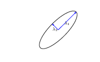
The data fit term of the Gaussian process is a quadratic loss centered
around zero. This has eliptical contours, the principal axes of which
are given by the covariance matrix.
\[E(\boldsymbol{ \theta}) =
\color{yellow}{\frac{1}{2}\log\det{\mathbf{K}}}+\color{cyan}{\frac{\mathbf{
y}^{\top}\mathbf{K}^{-1}\mathbf{ y}}{2}}\]
Exponentiated Quadratic Covariance
\[k(\mathbf{ x}, \mathbf{ x}^\prime) = \alpha
\exp\left(-\frac{\left\Vert \mathbf{ x}-\mathbf{ x}^\prime
\right\Vert_2^2}{2\ell^2}\right)\]
The exponentiated quadratic covariance function.
Where Did This Covariance Matrix Come From?
\[
k(\mathbf{ x}, \mathbf{ x}^\prime) = \alpha \exp\left(-\frac{\left\Vert
\mathbf{ x}- \mathbf{
x}^\prime\right\Vert^2_2}{2\ell^2}\right)\]
Covariance matrix is built using the inputs to the
function, \(\mathbf{ x}\) .
For the example above it was based on Euclidean
distance.
The covariance function is also know as a kernel.
Computing Covariance
❮
❯
Entrywise fill in of the covariance matrix from the covariance function.
Computing Covariance
❮
❯
Entrywise fill in of the covariance matrix from the covariance function.
Brownian Covariance
\[k(t, t^\prime)=\alpha \min(t,
t^\prime)\]
Brownian motion covariance function.
Where did this covariance matrix come from?
Markov Process
Visualization of inverse covariance (precision).
Precision matrix is sparse: only neighbours in matrix are
non-zero.
This reflects conditional independencies in
data.
In this case Markov structure.
Where did this covariance matrix come from?
Exponentiated Quadratic
Visualization of inverse covariance (precision).
Precision matrix is not sparse.
Each point is dependent on all the others.
In this case non-Markovian.
rbfprecisionSample
Covariance Functions
Markov Process
Visualization of inverse covariance (precision).
Precision matrix is sparse: only neighbours in matrix are
non-zero.
This reflects conditional independencies in data.
In this case Markov structure.
markovprecisionPlot
Exponential Covariance
\[k(\mathbf{ x}, \mathbf{ x}^\prime) = \alpha
\exp\left(-\frac{\left\Vert \mathbf{ x}-\mathbf{ x}^\prime
\right\Vert_2}{\ell}\right)\]
The exponential covariance function.
Basis Function Covariance
\[k(\mathbf{ x}, \mathbf{ x}^\prime) =
\boldsymbol{ \phi}(\mathbf{ x})^\top \boldsymbol{ \phi}(\mathbf{
x}^\prime)\]
A covariance function based on a non-linear basis given by \(\boldsymbol{ \phi}(\mathbf{ x})\) .
Degenerate Covariance Functions
RBF Basis Functions
\[
\phi_k(x) = \exp\left(-\frac{\left\Vert x-\mu_k
\right\Vert_2^{2}}{\ell^{2}}\right).
\]
\[
\boldsymbol{ \mu}= \begin{bmatrix} -1 \\ 0 \\ 1\end{bmatrix},
\]
\[
k\left(\mathbf{ x},\mathbf{ x}^{\prime}\right)=\alpha\boldsymbol{
\phi}(\mathbf{ x})^\top \boldsymbol{ \phi}(\mathbf{ x}^\prime).
\]
Bochners Theoerem
Given a positive finite Borel measure \(\mu\) on the real line \(\mathbb{R}\) , the Fourier transform \(Q\) of \(\mu\) is the continuous function \[
Q(t) = \int_{\mathbb{R}} e^{-itx} \text{d} \mu(x).
\] \(Q\) is continuous since
for a fixed \(x\) , the function \(e^{-itx}\) is continuous and periodic. The
function \(Q\) is a positive definite
function, i.e. the kernel \(k(x, x^\prime)=
Q(x^\prime - x)\) is positive definite.
Bochner’s theorem (Bochner, 1959) says the converse is
true, i.e. every positive definite function \(Q\) is the Fourier transform of a positive
finite Borel measure. A proof can be sketched as follows (Stein,
1999)
\[
f(\mathbf{ x}) = \sum_{i=1}^ny_i \delta(\mathbf{ x}-\mathbf{ x}_i),
\]
\[
F(\boldsymbol{\omega}) = \int_{-\infty}^\infty f(\mathbf{ x})
\exp\left(-i2\pi \boldsymbol{\omega}^\top \mathbf{ x}\right) \text{d}
\mathbf{ x}
\]
\[
F(\boldsymbol{\omega}) = \sum_{i=1}^ny_i\exp\left(-i 2\pi
\boldsymbol{\omega}^\top \mathbf{ x}_i\right)
\]
\[
F(\omega) = \int_{-\infty}^\infty f(t) \left[\cos(2\pi \omega t) - i
\sin(2\pi \omega t) \right]\text{d} t
\]
\[
\exp(ix) = \cos x + i\sin x
\] we can re-express this form as \[
F(\omega) = \int_{-\infty}^\infty f(t) \exp(-i 2\pi\omega)\text{d} t
\]
\[
f(t) = \int_{-\infty}^\infty F(\omega) \exp(2\pi\omega)\text{d} \omega.
\]
Sinc Covariance
\[k(\mathbf{ x}, \mathbf{ x}^\prime) = \alpha
\text{sinc}\left(\pi w r\right)\]
Sinc covariance function.
Matérn 3/2 Covariance
\[k(\mathbf{ x}, \mathbf{ x}^\prime) = \alpha
\left(1+\frac{\sqrt{3}\left\Vert \mathbf{ x}-\mathbf{ x}^\prime
\right\Vert_2}{\ell}\right)\exp\left(-\frac{\sqrt{3}\left\Vert \mathbf{
x}-\mathbf{ x}^\prime \right\Vert_2}{\ell}\right)\]
The Matérn 3/2 covariance function.
Matérn 5/2 Covariance
\[k(\mathbf{ x}, \mathbf{ x}^\prime) = \alpha
\left(1+\frac{\sqrt{5}\left\Vert \mathbf{ x}-\mathbf{ x}^\prime
\right\Vert_2}{\ell} + \frac{5\left\Vert \mathbf{ x}-\mathbf{ x}^\prime
\right\Vert_2^2}{3\ell^2}\right)\exp\left(-\frac{\sqrt{5}\left\Vert
\mathbf{ x}-\mathbf{ x}^\prime \right\Vert_2}{\ell}\right)\]
The Matérn 5/2 covariance function.
Rational Quadratic Covariance
\[k(\mathbf{ x}, \mathbf{ x}^\prime) = \alpha
\left(1+\frac{\left\Vert \mathbf{ x}-\mathbf{ x}^\prime
\right\Vert_2^2}{2 a \ell^2}\right)^{-a}\]
The rational quadratic covariance function.
Polynomial Covariance
\[k(\mathbf{ x}, \mathbf{ x}^\prime) =
\alpha(w \mathbf{ x}^\top\mathbf{ x}^\prime + b)^d\]
Polynomial covariance function.
Periodic Covariance
\[k(\mathbf{ x}, \mathbf{ x}^\prime) =
\alpha\exp\left(\frac{-2\sin(\pi rw)^2}{\ell^2}\right)\]
Periodic covariance function.
MLP Covariance
\[k(\mathbf{ x}, \mathbf{ x}^\prime) = \alpha
\arcsin\left(\frac{w \mathbf{ x}^\top \mathbf{ x}^\prime +
b}{\sqrt{\left(w \mathbf{ x}^\top \mathbf{ x}+ b + 1\right)\left(w
\left.\mathbf{ x}^\prime\right.^\top \mathbf{ x}^\prime + b +
1\right)}}\right)\]
The multi-layer perceptron covariance function. This is derived by
considering the infinite limit of a neural network with probit
activation functions.
RELU Covariance
\[k(\mathbf{ x}, \mathbf{ x}^\prime) =
\alpha \arcsin\left(\frac{w \mathbf{ x}^\top \mathbf{ x}^\prime + b}
{\sqrt{\left(w \mathbf{ x}^\top \mathbf{ x}+ b + 1\right)
\left(w \left.\mathbf{ x}^\prime\right.^\top \mathbf{ x}^\prime + b +
1\right)}}\right)\]
Rectified linear unit covariance function.
Additive Covariance
\[k_f(\mathbf{ x}, \mathbf{ x}^\prime) =
k_g(\mathbf{ x}, \mathbf{ x}^\prime) + k_h(\mathbf{ x}, \mathbf{
x}^\prime)\]
An additive covariance function formed by combining a linear and an
exponentiated quadratic covariance functions.
Product Covariance
\[k_f(\mathbf{ x}, \mathbf{ x}^\prime) =
k_g(\mathbf{ x}, \mathbf{ x}^\prime) k_h(\mathbf{ x}, \mathbf{
x}^\prime)\]
An product covariance function formed by combining a linear and an
exponentiated quadratic covariance functions.
Mauna Loa Data
Mauna Loa data shows carbon dioxide monthly average measurements from
the Mauna Loa Observatory in Hawaii.
Mauna Loa Test Data
Mauna Loa test data shows carbon dioxide monthly average measurements
from the Mauna Loa Observatory in Hawaii.
Mauna Loa Data GP
Gaussian process fit to the Mauna Loa Observatory data on CO2
concentrations.
Box Jenkins Airline Passenger Data
Mauna Loa Data
Box-Jenkins data set on airline passenger numbers.
Box-Jenkins Airline PassengerData GP
Gaussian process fit to the Box-Jenkins airline passenger data.
Box-Jenkins Airline Spectral Mixture
Spectral mixture GP as applied to the Box-Jenkins airline data.
Mauna Loa Spectral Mixture
Spectral mixture GP as applied to the Mauna Loa Observatory carbon
dioxide concentration data.