Week 2: Gaussian Distributions to Processes

[Powerpoint][jupyter][google colab][reveal]

Abstract:

In this sesson we go from the Gaussian distribution to the Gaussian process and in doing so we move from a finite system to an infinite system.

%pip install gpy

GPy: A Gaussian Process Framework in Python

Gaussian processes are a flexible tool for non-parametric analysis with uncertainty. The GPy software was started in Sheffield to provide a easy to use interface to GPs. One which allowed the user to focus on the modelling rather than the mathematics.

Figure: GPy is a BSD licensed software code base for implementing Gaussian process models in Python. It is designed for teaching and modelling. We welcome contributions which can be made through the GitHub repository https://github.com/SheffieldML/GPy

GPy is a BSD licensed software code base for implementing Gaussian process models in python. This allows GPs to be combined with a wide variety of software libraries.

The software itself is available on GitHub and the team welcomes contributions.

The aim for GPy is to be a probabilistic-style programming language, i.e., you specify the model rather than the algorithm. As well as a large range of covariance functions the software allows for non-Gaussian likelihoods, multivariate outputs, dimensionality reduction and approximations for larger data sets.

The documentation for GPy can be found here.

Two Dimensional Gaussian

Consider the distribution of height (in meters) of an adult male human population. We will approximate the marginal density of heights as a Gaussian density with mean given by \(1.7\text{m}\) and a standard deviation of \(0.15\text{m}\), implying a variance of \(\sigma^2=0.0225\), \[ p(h) \sim \mathcal{N}\left(1.7,0.0225\right). \] Similarly, we assume that weights of the population are distributed a Gaussian density with a mean of \(75 \text{kg}\) and a standard deviation of \(6 kg\) (implying a variance of 36), \[ p(w) \sim \mathcal{N}\left(75,36\right). \]

Figure: Gaussian distributions for height and weight.

Independence Assumption

First of all, we make an independence assumption, we assume that height and weight are independent. The definition of probabilistic independence is that the joint density, \(p(w, h)\), factorizes into its marginal densities, \[ p(w, h) = p(w)p(h). \] Given this assumption we can sample from the joint distribution by independently sampling weights and heights.

Figure: Samples from independent Gaussian variables that might represent heights and weights.

In reality height and weight are not independent. Taller people tend on average to be heavier, and heavier people are likely to be taller. This is reflected by the body mass index. A ratio suggested by one of the fathers of statistics, Adolphe Quetelet. Quetelet was interested in the notion of the average man and collected various statistics about people. He defined the BMI to be, \[ \text{BMI} = \frac{w}{h^2} \]To deal with this dependence we now introduce the notion of correlation to the multivariate Gaussian density.

Sampling Two Dimensional Variables

Figure: Samples from correlated Gaussian variables that might represent heights and weights.

Independent Gaussians

\[ p(w, h) = p(w)p(h) \]

\[ p(w, h) = \frac{1}{\sqrt{2\pi \sigma_1^2}\sqrt{2\pi\sigma_2^2}} \exp\left(-\frac{1}{2}\left(\frac{(w-\mu_1)^2}{\sigma_1^2} + \frac{(h-\mu_2)^2}{\sigma_2^2}\right)\right) \]

\[ p(w, h) = \frac{1}{\sqrt{2\pi\sigma_1^22\pi\sigma_2^2}} \exp\left(-\frac{1}{2}\left(\begin{bmatrix}w \\ h\end{bmatrix} - \begin{bmatrix}\mu_1 \\ \mu_2\end{bmatrix}\right)^\top\begin{bmatrix}\sigma_1^2& 0\\0&\sigma_2^2\end{bmatrix}^{-1}\left(\begin{bmatrix}w \\ h\end{bmatrix} - \begin{bmatrix}\mu_1 \\ \mu_2\end{bmatrix}\right)\right) \]

\[ p(\mathbf{ y}) = \frac{1}{\det{2\pi \mathbf{D}}^{\frac{1}{2}}} \exp\left(-\frac{1}{2}(\mathbf{ y}- \boldsymbol{ \mu})^\top\mathbf{D}^{-1}(\mathbf{ y}- \boldsymbol{ \mu})\right) \]

Correlated Gaussian

Form correlated from original by rotating the data space using matrix \(\mathbf{R}\).

\[ p(\mathbf{ y}) = \frac{1}{\det{2\pi\mathbf{D}}^{\frac{1}{2}}} \exp\left(-\frac{1}{2}(\mathbf{ y}- \boldsymbol{ \mu})^\top\mathbf{D}^{-1}(\mathbf{ y}- \boldsymbol{ \mu})\right) \]

\[ p(\mathbf{ y}) = \frac{1}{\det{2\pi\mathbf{D}}^{\frac{1}{2}}} \exp\left(-\frac{1}{2}(\mathbf{R}^\top\mathbf{ y}- \mathbf{R}^\top\boldsymbol{ \mu})^\top\mathbf{D}^{-1}(\mathbf{R}^\top\mathbf{ y}- \mathbf{R}^\top\boldsymbol{ \mu})\right) \]

\[ p(\mathbf{ y}) = \frac{1}{\det{2\pi\mathbf{D}}^{\frac{1}{2}}} \exp\left(-\frac{1}{2}(\mathbf{ y}- \boldsymbol{ \mu})^\top\mathbf{R}\mathbf{D}^{-1}\mathbf{R}^\top(\mathbf{ y}- \boldsymbol{ \mu})\right) \] this gives a covariance matrix: \[ \mathbf{C}^{-1} = \mathbf{R}\mathbf{D}^{-1} \mathbf{R}^\top \]

\[ p(\mathbf{ y}) = \frac{1}{\det{2\pi\mathbf{C}}^{\frac{1}{2}}} \exp\left(-\frac{1}{2}(\mathbf{ y}- \boldsymbol{ \mu})^\top\mathbf{C}^{-1} (\mathbf{ y}- \boldsymbol{ \mu})\right) \] this gives a covariance matrix: \[ \mathbf{C}= \mathbf{R}\mathbf{D} \mathbf{R}^\top \]

Let’s first of all review the properties of the multivariate Gaussian distribution that make linear Gaussian models easier to deal with. We’ll return to the, perhaps surprising, result on the parameters within the nonlinearity, \(\boldsymbol{ \theta}\), shortly.

To work with linear Gaussian models, to find the marginal likelihood all you need to know is the following rules. If \[ \mathbf{ y}= \mathbf{W}\mathbf{ x}+ \boldsymbol{ \epsilon}, \] where \(\mathbf{ y}\), \(\mathbf{ x}\) and \(\boldsymbol{ \epsilon}\) are vectors and we assume that \(\mathbf{ x}\) and \(\boldsymbol{ \epsilon}\) are drawn from multivariate Gaussians, \[ \begin{align} \mathbf{ x}& \sim \mathcal{N}\left(\boldsymbol{ \mu},\mathbf{C}\right)\\ \boldsymbol{ \epsilon}& \sim \mathcal{N}\left(\mathbf{0},\boldsymbol{ \Sigma}\right) \end{align} \] then we know that \(\mathbf{ y}\) is also drawn from a multivariate Gaussian with, \[ \mathbf{ y}\sim \mathcal{N}\left(\mathbf{W}\boldsymbol{ \mu},\mathbf{W}\mathbf{C}\mathbf{W}^\top + \boldsymbol{ \Sigma}\right). \]

With appropriately defined covariance, \(\boldsymbol{ \Sigma}\), this is actually the marginal likelihood for Factor Analysis, or Probabilistic Principal Component Analysis (Tipping and Bishop, 1999), because we integrated out the inputs (or latent variables they would be called in that case).

Linear Model Overview

However, we are focussing on what happens in models which are non-linear in the inputs, whereas the above would be linear in the inputs. To consider these, we introduce a matrix, called the design matrix. We set each activation function computed at each data point to be \[ \phi_{i,j} = \phi(\mathbf{ w}^{(1)}_{j}, \mathbf{ x}_{i}) \] and define the matrix of activations (known as the design matrix in statistics) to be, \[ \boldsymbol{ \Phi}= \begin{bmatrix} \phi_{1, 1} & \phi_{1, 2} & \dots & \phi_{1, h} \\ \phi_{1, 2} & \phi_{1, 2} & \dots & \phi_{1, n} \\ \vdots & \vdots & \ddots & \vdots \\ \phi_{n, 1} & \phi_{n, 2} & \dots & \phi_{n, h} \end{bmatrix}. \] By convention this matrix always has \(n\) rows and \(h\) columns, now if we define the vector of all noise corruptions, \(\boldsymbol{ \epsilon}= \left[\epsilon_1, \dots \epsilon_n\right]^\top\).

If we define the prior distribution over the vector \(\mathbf{ w}\) to be Gaussian, \[ \mathbf{ w}\sim \mathcal{N}\left(\mathbf{0},\alpha\mathbf{I}\right), \] then we can use rules of multivariate Gaussians to see that, \[ \mathbf{ y}\sim \mathcal{N}\left(\mathbf{0},\alpha \boldsymbol{ \Phi}\boldsymbol{ \Phi}^\top + \sigma^2 \mathbf{I}\right). \]

In other words, our training data is distributed as a multivariate Gaussian, with zero mean and a covariance given by \[ \mathbf{K}= \alpha \boldsymbol{ \Phi}\boldsymbol{ \Phi}^\top + \sigma^2 \mathbf{I}. \]

This is an \(n\times n\) size matrix. Its elements are in the form of a function. The maths shows that any element, index by \(i\) and \(j\), is a function only of inputs associated with data points \(i\) and \(j\), \(\mathbf{ y}_i\), \(\mathbf{ y}_j\). \(k_{i,j} = k\left(\mathbf{ x}_i, \mathbf{ x}_j\right)\)

If we look at the portion of this function associated only with \(f(\cdot)\), i.e. we remove the noise, then we can write down the covariance associated with our neural network, \[ k_f\left(\mathbf{ x}_i, \mathbf{ x}_j\right) = \alpha \boldsymbol{ \phi}\left(\mathbf{W}_1, \mathbf{ x}_i\right)^\top \boldsymbol{ \phi}\left(\mathbf{W}_1, \mathbf{ x}_j\right) \] so the elements of the covariance or kernel matrix are formed by inner products of the rows of the design matrix.

Gaussian Process

This is the essence of a Gaussian process. Instead of making assumptions about our density over each data point, \(y_i\) as i.i.d. we make a joint Gaussian assumption over our data. The covariance matrix is now a function of both the parameters of the activation function, \(\mathbf{V}\), and the input variables, \(\mathbf{X}\). This comes about through integrating out the parameters of the model, \(\mathbf{ w}\).

Basis Functions

We can basically put anything inside the basis functions, and many people do. These can be deep kernels (Cho and Saul, 2009) or we can learn the parameters of a convolutional neural network inside there.

Viewing a neural network in this way is also what allows us to beform sensible batch normalizations (Ioffe and Szegedy, 2015).

Bayesian Inference by Rejection Sampling

One view of Bayesian inference is to assume we are given a mechanism for generating samples, where we assume that mechanism is representing an accurate view on the way we believe the world works.

This mechanism is known as our prior belief.

We combine our prior belief with our observations of the real world by discarding all those prior samples that are inconsistent with our observations. The likelihood defines mathematically what we mean by inconsistent with the observations. The higher the noise level in the likelihood, the looser the notion of consistent.

The samples that remain are samples from the posterior.

This approach to Bayesian inference is closely related to two sampling techniques known as rejection sampling and importance sampling. It is realized in practice in an approach known as approximate Bayesian computation (ABC) or likelihood-free inference.

In practice, the algorithm is often too slow to be practical, because most samples will be inconsistent with the observations and as a result the mechanism must be operated many times to obtain a few posterior samples.

However, in the Gaussian process case, when the likelihood also assumes Gaussian noise, we can operate this mechanism mathematically, and obtain the posterior density analytically. This is the benefit of Gaussian processes.

First, we will load in two python functions for computing the covariance function.

Next, we sample from a multivariate normal density (a multivariate Gaussian), using the covariance function as the covariance matrix.

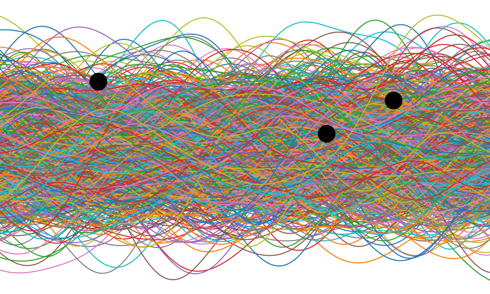
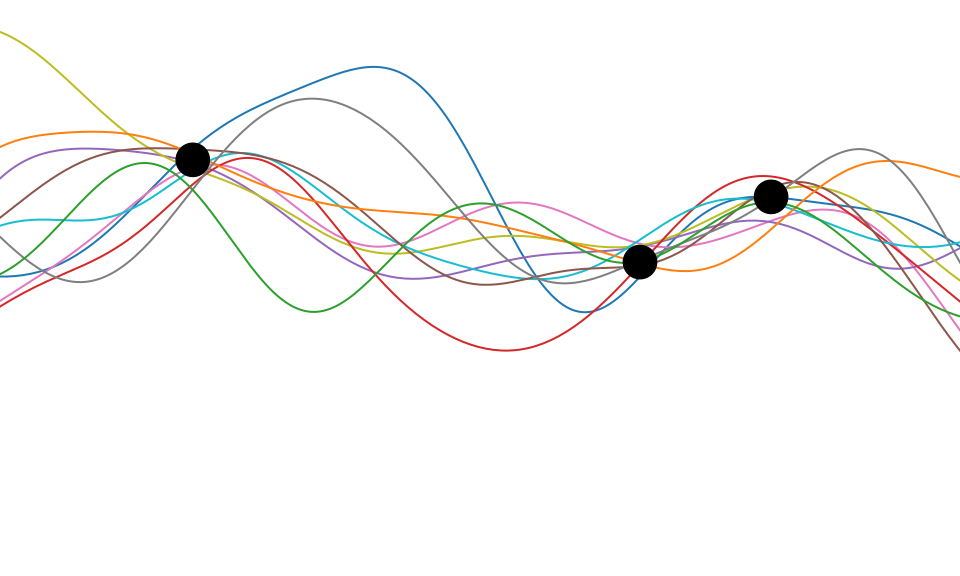
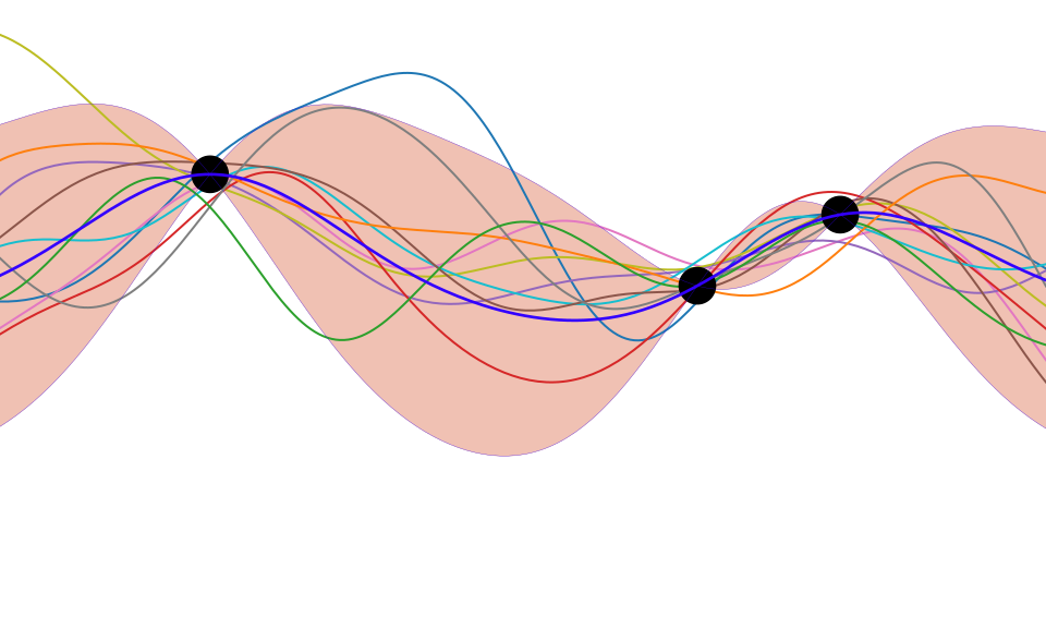
Figure: One view of Bayesian inference is we have a machine for generating samples (the prior), and we discard all samples inconsistent with our data, leaving the samples of interest (the posterior). This is a rejection sampling view of Bayesian inference. The Gaussian process allows us to do this analytically by multiplying the prior by the likelihood.

Sampling a Function

We will consider a Gaussian distribution with a particular structure of covariance matrix. We will generate one sample from a 25-dimensional Gaussian density. \[ \mathbf{ f}=\left[f_{1},f_{2}\dots f_{25}\right]. \] in the figure below we plot these data on the \(y\)-axis against their indices on the \(x\)-axis.

import mlai

from mlai import Kernel

import mlai

from mlai import polynomial_cov

import mlai

from mlai import exponentiated_quadratic

Figure: A 25 dimensional correlated random variable (values ploted against index)

Sampling a Function from a Gaussian

Figure: The joint Gaussian over \(f_1\) and \(f_2\) along with the conditional distribution of \(f_2\) given \(f_1\)

Joint Density of \(f_1\) and \(f_2\)

Figure: The joint Gaussian over \(f_1\) and \(f_2\) along with the conditional distribution of \(f_2\) given \(f_1\)

Uluru

Figure: Uluru, the sacred rock in Australia. If we think of it as a probability density, viewing it from this side gives us one marginal from the density. Figuratively speaking, slicing through the rock would give a conditional density.

When viewing these contour plots, I sometimes find it helpful to think of Uluru, the prominent rock formation in Australia. The rock rises above the surface of the plane, just like a probability density rising above the zero line. The rock is three dimensional, but when we view Uluru from the classical position, we are looking at one side of it. This is equivalent to viewing the marginal density.

The joint density can be viewed from above, using contours. The conditional density is equivalent to slicing the rock. Uluru is a holy rock, so this has to be an imaginary slice. Imagine we cut down a vertical plane orthogonal to our view point (e.g. coming across our view point). This would give a profile of the rock, which when renormalized, would give us the conditional distribution, the value of conditioning would be the location of the slice in the direction we are facing.

Prediction with Correlated Gaussians

Of course in practice, rather than manipulating mountains physically, the advantage of the Gaussian density is that we can perform these manipulations mathematically.

Prediction of \(f_2\) given \(f_1\) requires the conditional density, \(p(f_2|f_1)\).Another remarkable property of the Gaussian density is that this conditional distribution is also guaranteed to be a Gaussian density. It has the form, \[ p(f_2|f_1) = \mathcal{N}\left(f_2|\frac{k_{1, 2}}{k_{1, 1}}f_1, k_{2, 2} - \frac{k_{1,2}^2}{k_{1,1}}\right) \]where we have assumed that the covariance of the original joint density was given by \[ \mathbf{K}= \begin{bmatrix} k_{1, 1} & k_{1, 2}\\ k_{2, 1} & k_{2, 2}.\end{bmatrix} \]

Using these formulae we can determine the conditional density for any of the elements of our vector \(\mathbf{ f}\). For example, the variable \(f_8\) is less correlated with \(f_1\) than \(f_2\). If we consider this variable we see the conditional density is more diffuse.

Joint Density of \(f_1\) and \(f_8\)

Figure: Sample from the joint Gaussian model, points indexed by 1 and 8 highlighted.

Prediction of \(f_{8}\) from \(f_{1}\)

Figure: The joint Gaussian over \(f_1\) and \(f_8\) along with the conditional distribution of \(f_8\) given \(f_1\)

• The single contour of the Gaussian density represents the joint distribution, \(p(f_1, f_8)\)

. . .

• We observe a value for \(f_1=-?\)

. . .

• Conditional density: \(p(f_8|f_1=?)\).

• Prediction of \(\mathbf{ f}_*\) from \(\mathbf{ f}\) requires multivariate conditional density.

• Multivariate conditional density is also Gaussian. \[ p(\mathbf{ f}_*|\mathbf{ f}) = {\mathcal{N}\left(\mathbf{ f}_*|\mathbf{K}_{*,\mathbf{ f}}\mathbf{K}_{\mathbf{ f},\mathbf{ f}}^{-1}\mathbf{ f},\mathbf{K}_{*,*}-\mathbf{K}_{*,\mathbf{ f}} \mathbf{K}_{\mathbf{ f},\mathbf{ f}}^{-1}\mathbf{K}_{\mathbf{ f},*}\right)} \]

• Here covariance of joint density is given by \[ \mathbf{K}= \begin{bmatrix} \mathbf{K}_{\mathbf{ f}, \mathbf{ f}} & \mathbf{K}_{*, \mathbf{ f}}\\ \mathbf{K}_{\mathbf{ f}, *} & \mathbf{K}_{*, *}\end{bmatrix} \]

• Prediction of \(\mathbf{ f}_*\) from \(\mathbf{ f}\) requires multivariate conditional density.

• Multivariate conditional density is also Gaussian. \[ p(\mathbf{ f}_*|\mathbf{ f}) = {\mathcal{N}\left(\mathbf{ f}_*|\boldsymbol{ \mu},\boldsymbol{ \Sigma}\right)} \] \[ \boldsymbol{ \mu}= \mathbf{K}_{*,\mathbf{ f}}\mathbf{K}_{\mathbf{ f},\mathbf{ f}}^{-1}\mathbf{ f} \] \[ \boldsymbol{ \Sigma}= \mathbf{K}_{*,*}-\mathbf{K}_{*,\mathbf{ f}} \mathbf{K}_{\mathbf{ f},\mathbf{ f}}^{-1}\mathbf{K}_{\mathbf{ f},*} \]

• Here covariance of joint density is given by \[ \mathbf{K}= \begin{bmatrix} \mathbf{K}_{\mathbf{ f}, \mathbf{ f}} & \mathbf{K}_{*, \mathbf{ f}}\\ \mathbf{K}_{\mathbf{ f}, *} & \mathbf{K}_{*, *}\end{bmatrix} \]

Where Did This Covariance Matrix Come From?

\[ k(\mathbf{ x}, \mathbf{ x}^\prime) = \alpha \exp\left(-\frac{\left\Vert \mathbf{ x}- \mathbf{ x}^\prime\right\Vert^2_2}{2\ell^2}\right)\]

Figure: Entrywise fill in of the covariance matrix from the covariance function.

Figure: Entrywise fill in of the covariance matrix from the covariance function.

Figure: Entrywise fill in of the covariance matrix from the covariance function.

Polynomial Covariance

Figure: Polynomial covariance function.

Degenerate Covariance Functions

Any linear basis function can also be incorporated into a covariance function. For example, an RBF network is a type of neural network with a set of radial basis functions. Meaning, the basis funciton is radially symmetric. These basis functions take the form, \[ \phi_k(x) = \exp\left(-\frac{\left\Vert x-\mu_k \right\Vert_2^{2}}{\ell^{2}}\right). \] Given a set of parameters, \[ \boldsymbol{ \mu}= \begin{bmatrix} -1 \\ 0 \\ 1\end{bmatrix}, \] we can construct the corresponding covariance function, which has the form, \[ k\left(\mathbf{ x},\mathbf{ x}^{\prime}\right)=\alpha\boldsymbol{ \phi}(\mathbf{ x})^\top \boldsymbol{ \phi}(\mathbf{ x}^\prime). \]

Basis Function Covariance

The fixed basis function covariance just comes from the properties of a multivariate Gaussian, if we decide \[ \mathbf{ f}=\boldsymbol{ \Phi}\mathbf{ w} \] and then we assume \[ \mathbf{ w}\sim \mathcal{N}\left(\mathbf{0},\alpha\mathbf{I}\right) \] then it follows from the properties of a multivariate Gaussian that \[ \mathbf{ f}\sim \mathcal{N}\left(\mathbf{0},\alpha\boldsymbol{ \Phi}\boldsymbol{ \Phi}^\top\right) \] meaning that the vector of observations from the function is jointly distributed as a Gaussian process and the covariance matrix is \(\mathbf{K}= \alpha\boldsymbol{ \Phi}\boldsymbol{ \Phi}^\top\), each element of the covariance matrix can then be found as the inner product between two rows of the basis funciton matrix.

import mlai

from mlai import basis_cov

import mlai

from mlai import radial

Figure: A covariance function based on a non-linear basis given by \(\boldsymbol{ \phi}(\mathbf{ x})\).

Selecting Number and Location of Basis

In practice for a basis function model we need to choose both 1. the location of the basis functions 2. the number of basis functions

One very clever of finessing this problem is to choose to have infinite basis functions and place them everywhere. To show how this is possible, we will consider a one dimensional system, \(x\), which should give the intuition of how to do this. However, these ideas also extend to multidimensional systems as shown in, for example, Williams (n.d.) and Neal (1994).

We consider a one dimensional set up with exponentiated quadratic basis functions, \[ \phi_k(x_i) = \exp\left(\frac{\left\Vert x_i - \mu_k \right\Vert_2^2}{2\ell^2}\right) \]

To place these basis functions, we first define the basis function centers in terms of a starting point on the left of our input, \(a\), and a finishing point, \(b\). The gap between basis is given by \(\Delta\mu\). The location of each basis is then given by \[\mu_k = a+\Delta\mu\cdot (k-1).\] The covariance function can then be given as \[ k\left(x_i,x_j\right) = \sum_{k=1}^m\phi_k(x_i)\phi_k(x_j) \] \[\begin{aligned} k\left(x_i,x_j\right) = &\alpha^\prime\Delta\mu\sum_{k=1}^{m} \exp\Bigg( -\frac{x_i^2 + x_j^2}{2\ell^2}\\ & - \frac{2\left(a+\Delta\mu\cdot (k-1)\right) \left(x_i+x_j\right) + 2\left(a+\Delta\mu\cdot (k-1)\right)^2}{2\ell^2} \Bigg) \end{aligned}\] where we’ve also scaled the variance of the process by \(\Delta\mu\).

A consequence of our definition is that the first and last basis function locations are given by \[ \mu_1=a \ \text{and}\ \mu_m=b \ \text{so}\ b= a+ \Delta\mu\cdot(m-1) \] This implies that the distance between \(b\) and \(a\) is given by \[ b-a = \Delta\mu(m-1) \] and since the basis functions are separated by \(\Delta\mu\) the number of basis functions is given by \[ m= \frac{b-a}{\Delta \mu} + 1 \] The next step is to take the limit as \(\Delta\mu\rightarrow 0\) so \(m\rightarrow \infty\) where we have used \(a + k\cdot\Delta\mu\rightarrow \mu\).

Performing the integration gives \[\begin{aligned} k(x_i,&x_j) = \alpha^\prime \sqrt{\pi\ell^2} \exp\left( -\frac{\left(x_i-x_j\right)^2}{4\ell^2}\right)\\ &\times \frac{1}{2}\left[\text{erf}\left(\frac{\left(b - \frac{1}{2}\left(x_i + x_j\right)\right)}{\ell} \right)- \text{erf}\left(\frac{\left(a - \frac{1}{2}\left(x_i + x_j\right)\right)}{\ell} \right)\right], \end{aligned}\]Now we take the limit as \(a\rightarrow -\infty\) and \(b\rightarrow \infty\) \[k\left(x_i,x_j\right) = \alpha\exp\left( -\frac{\left(x_i-x_j\right)^2}{4\ell^2}\right).\] where \(\alpha=\alpha^\prime \sqrt{\pi\ell^2}\).

In conclusion, an RBF model with infinite basis functions is a Gaussian process with the exponentiated quadratic covariance function \[k\left(x_i,x_j\right) = \alpha \exp\left( -\frac{\left(x_i-x_j\right)^2}{4\ell^2}\right).\]

Note that while the functional form of the basis function and the covariance function are similar, in general if we repeated this analysis for other basis functions the covariance function will have a very different form. For example the error function, \(\text{erf}(\cdot)\), results in an \(\asin(\cdot)\) form. See Williams (n.d.) for more details.

Thanks!

For more information on these subjects and more you might want to check the following resources.

• twitter: @lawrennd
• podcast: The Talking Machines
• newspaper: Guardian Profile Page
• blog: http://inverseprobability.com

References