Gaussian Distributions to Processes

GPy: A Gaussian Process Framework in Python

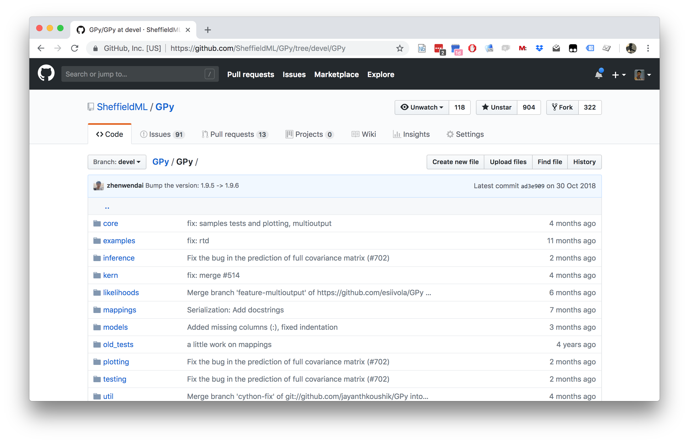
GPy: A Gaussian Process Framework in Python

• BSD Licensed software base.
• Wide availability of libraries, ‘modern’ scripting language.
• Allows us to set projects to undergraduates in Comp Sci that use GPs.
• Available through GitHub https://github.com/SheffieldML/GPy
• Reproducible Research with Jupyter Notebook.

Features

• Probabilistic-style programming (specify the model, not the algorithm).
• Non-Gaussian likelihoods.
• Multivariate outputs.
• Dimensionality reduction.
• Approximations for large data sets.

Two Dimensional Gaussian Distribution

Two Dimensional Gaussian

• Consider height, \(h/m\) and weight, \(w/kg\).
• Could sample height from a distribution: \[ p(h) \sim \mathcal{N}\left(1.7,0.0225\right). \]
• And similarly weight: \[ p(w) \sim \mathcal{N}\left(75,36\right). \]

Height and Weight Models

Independence Assumption

• We assume height and weight are independent.

  \[ p(w, h) = p(w)p(h). \]

Sampling Two Dimensional Variables

❮ ❯

Body Mass Index

• In reality they are dependent (body mass index) \(= \frac{w}{h^2}\).
• To deal with this dependence we introduce correlated multivariate Gaussians.

Sampling Two Dimensional Variables

❮ ❯

Independent Gaussians

\[ p(w, h) = p(w)p(h) \]

Independent Gaussians

\[ p(w, h) = \frac{1}{\sqrt{2\pi \sigma_1^2}\sqrt{2\pi\sigma_2^2}} \exp\left(-\frac{1}{2}\left(\frac{(w-\mu_1)^2}{\sigma_1^2} + \frac{(h-\mu_2)^2}{\sigma_2^2}\right)\right) \]

Independent Gaussians

\[ p(w, h) = \frac{1}{\sqrt{2\pi\sigma_1^22\pi\sigma_2^2}} \exp\left(-\frac{1}{2}\left(\begin{bmatrix}w \\ h\end{bmatrix} - \begin{bmatrix}\mu_1 \\ \mu_2\end{bmatrix}\right)^\top\begin{bmatrix}\sigma_1^2& 0\\0&\sigma_2^2\end{bmatrix}^{-1}\left(\begin{bmatrix}w \\ h\end{bmatrix} - \begin{bmatrix}\mu_1 \\ \mu_2\end{bmatrix}\right)\right) \]

Independent Gaussians

\[ p(\mathbf{ y}) = \frac{1}{\det{2\pi \mathbf{D}}^{\frac{1}{2}}} \exp\left(-\frac{1}{2}(\mathbf{ y}- \boldsymbol{ \mu})^\top\mathbf{D}^{-1}(\mathbf{ y}- \boldsymbol{ \mu})\right) \]

Correlated Gaussian

Form correlated from original by rotating the data space using matrix \(\mathbf{R}\).

\[ p(\mathbf{ y}) = \frac{1}{\det{2\pi\mathbf{D}}^{\frac{1}{2}}} \exp\left(-\frac{1}{2}(\mathbf{ y}- \boldsymbol{ \mu})^\top\mathbf{D}^{-1}(\mathbf{ y}- \boldsymbol{ \mu})\right) \]

Correlated Gaussian

Form correlated from original by rotating the data space using matrix \(\mathbf{R}\).

\[ p(\mathbf{ y}) = \frac{1}{\det{2\pi\mathbf{D}}^{\frac{1}{2}}} \exp\left(-\frac{1}{2}(\mathbf{R}^\top\mathbf{ y}- \mathbf{R}^\top\boldsymbol{ \mu})^\top\mathbf{D}^{-1}(\mathbf{R}^\top\mathbf{ y}- \mathbf{R}^\top\boldsymbol{ \mu})\right) \]

Correlated Gaussian

Form correlated from original by rotating the data space using matrix \(\mathbf{R}\).

\[ p(\mathbf{ y}) = \frac{1}{\det{2\pi\mathbf{D}}^{\frac{1}{2}}} \exp\left(-\frac{1}{2}(\mathbf{ y}- \boldsymbol{ \mu})^\top\mathbf{R}\mathbf{D}^{-1}\mathbf{R}^\top(\mathbf{ y}- \boldsymbol{ \mu})\right) \] this gives a covariance matrix: \[ \mathbf{C}^{-1} = \mathbf{R}\mathbf{D}^{-1} \mathbf{R}^\top \]

Correlated Gaussian

Form correlated from original by rotating the data space using matrix \(\mathbf{R}\).

\[ p(\mathbf{ y}) = \frac{1}{\det{2\pi\mathbf{C}}^{\frac{1}{2}}} \exp\left(-\frac{1}{2}(\mathbf{ y}- \boldsymbol{ \mu})^\top\mathbf{C}^{-1} (\mathbf{ y}- \boldsymbol{ \mu})\right) \] this gives a covariance matrix: \[ \mathbf{C}= \mathbf{R}\mathbf{D} \mathbf{R}^\top \]

Multivariate Gaussian Properties

Recall Univariate Gaussian Properties

Recall Univariate Gaussian Properties

2. Scaling a Gaussian leads to a Gaussian.

Multivariate Consequence

\[\mathbf{ x}\sim \mathcal{N}\left(\boldsymbol{ \mu},\mathbf{C}\right)\]

Linear Gaussian Models

Gaussian processes are initially of interest because 1. linear Gaussian models are easier to deal with 2. Even the parameters within the process can be handled, by considering a particular limit.

Multivariate Gaussian Properties

• If \[ \mathbf{ y}= \mathbf{W}\mathbf{ x}+ \boldsymbol{ \epsilon}, \]

• Assume \[ \begin{align} \mathbf{ x}& \sim \mathcal{N}\left(\boldsymbol{ \mu},\mathbf{C}\right)\\ \boldsymbol{ \epsilon}& \sim \mathcal{N}\left(\mathbf{0},\boldsymbol{ \Sigma}\right) \end{align} \]

• Then \[ \mathbf{ y}\sim \mathcal{N}\left(\mathbf{W}\boldsymbol{ \mu},\mathbf{W}\mathbf{C}\mathbf{W}^\top + \boldsymbol{ \Sigma}\right). \] If \(\boldsymbol{ \Sigma}=\sigma^2\mathbf{I}\), this is Probabilistic PCA (Tipping and Bishop, 1999).

Linear Model Overview

• Set each activation function computed at each data point to be

\[ \phi_{i,j} = \phi(\mathbf{ w}^{(1)}_{j}, \mathbf{ x}_{i}) \] Define design matrix \[ \boldsymbol{ \Phi}= \begin{bmatrix} \phi_{1, 1} & \phi_{1, 2} & \dots & \phi_{1, h} \\ \phi_{1, 2} & \phi_{1, 2} & \dots & \phi_{1, n} \\ \vdots & \vdots & \ddots & \vdots \\ \phi_{n, 1} & \phi_{n, 2} & \dots & \phi_{n, h} \end{bmatrix}. \]

Matrix Representation of a Neural Network

\[y\left(\mathbf{ x}\right) = \boldsymbol{ \phi}\left(\mathbf{ x}\right)^\top \mathbf{ w}+ \epsilon\]

Multivariate Gaussian Properties

• If \[ \mathbf{ y}= \mathbf{W}\mathbf{ x}+ \boldsymbol{ \epsilon}, \]

• Assume \[ \begin{align} \mathbf{ x}& \sim \mathcal{N}\left(\boldsymbol{ \mu},\mathbf{C}\right)\\ \boldsymbol{ \epsilon}& \sim \mathcal{N}\left(\mathbf{0},\boldsymbol{ \Sigma}\right) \end{align} \]

• Then \[ \mathbf{ y}\sim \mathcal{N}\left(\mathbf{W}\boldsymbol{ \mu},\mathbf{W}\mathbf{C}\mathbf{W}^\top + \boldsymbol{ \Sigma}\right). \] If \(\boldsymbol{ \Sigma}=\sigma^2\mathbf{I}\), this is Probabilistic PCA (Tipping and Bishop, 1999).

Prior Density

• Define \[ \mathbf{ w}\sim \mathcal{N}\left(\mathbf{0},\alpha\mathbf{I}\right), \]
• Rules of multivariate Gaussians to see that, \[ \mathbf{ y}\sim \mathcal{N}\left(\mathbf{0},\alpha \boldsymbol{ \Phi}\boldsymbol{ \Phi}^\top + \sigma^2 \mathbf{I}\right). \]

\[ \mathbf{K}= \alpha \boldsymbol{ \Phi}\boldsymbol{ \Phi}^\top + \sigma^2 \mathbf{I}. \]

Joint Gaussian Density

• Elements are a function \(k_{i,j} = k\left(\mathbf{ x}_i, \mathbf{ x}_j\right)\)

\[ \mathbf{K}= \alpha \boldsymbol{ \Phi}\boldsymbol{ \Phi}^\top + \sigma^2 \mathbf{I}. \]

Covariance Function

\[ k_f\left(\mathbf{ x}_i, \mathbf{ x}_j\right) = \alpha \boldsymbol{ \phi}\left(\mathbf{W}_1, \mathbf{ x}_i\right)^\top \boldsymbol{ \phi}\left(\mathbf{W}_1, \mathbf{ x}_j\right) \]

• formed by inner products of the rows of the design matrix.

Gaussian Process

• Instead of making assumptions about our density over each data point, \(y_i\) as i.i.d.

• make a joint Gaussian assumption over our data.

• covariance matrix is now a function of both the parameters of the activation function, \(\mathbf{W}_1\), and the input variables, \(\mathbf{X}\).

• Arises from integrating out \(\mathbf{ w}^{(2)}\).

Basis Functions

• Can be very complex, such as deep kernels, (Cho and Saul, 2009) or could even put a convolutional neural network inside.
• Viewing a neural network in this way is also what allows us to beform sensible batch normalizations (Ioffe and Szegedy, 2015).

Distributions over Functions

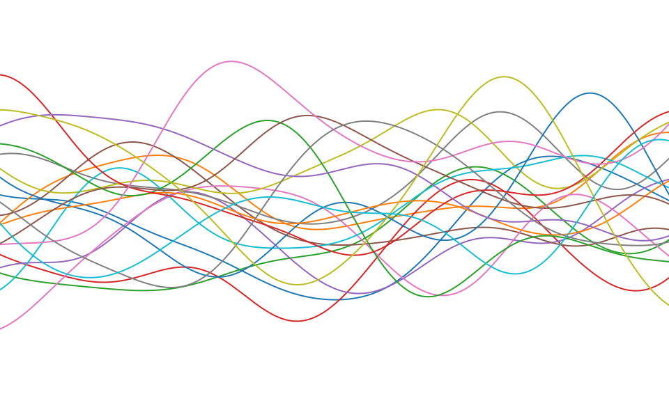
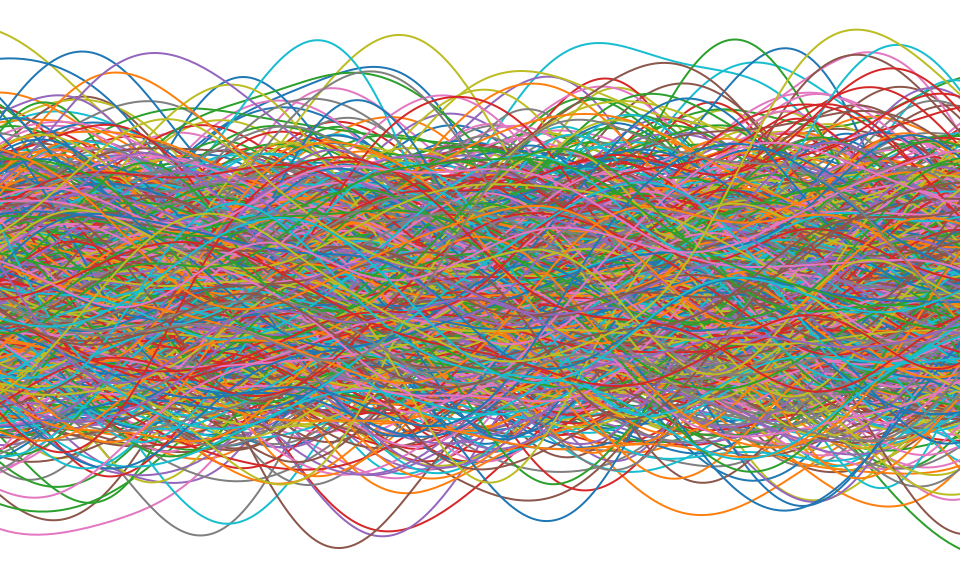
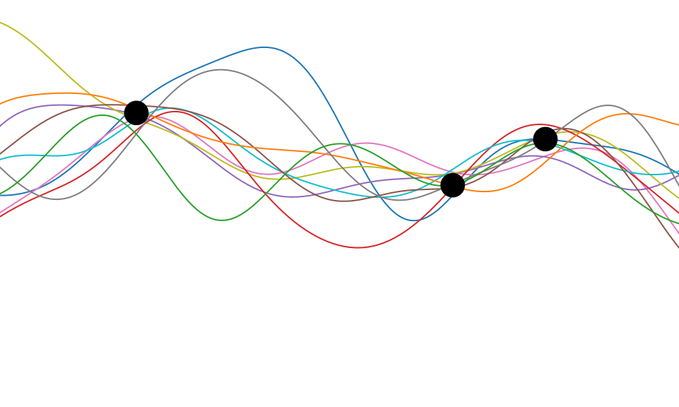
Sampling a Function

Multi-variate Gaussians

• We will consider a Gaussian with a particular structure of covariance matrix.
• Generate a single sample from this 25 dimensional Gaussian density, \[ \mathbf{ f}=\left[f_{1},f_{2}\dots f_{25}\right]. \]
• We will plot these points against their index.

Gaussian Distribution Sample

❮ ❯

Sampling a Function from a Gaussian

❮ ❯

Joint Density of \(f_1\) and \(f_2\)

Prediction of \(f_{2}\) from \(f_{1}\)

❮ ❯

Uluru

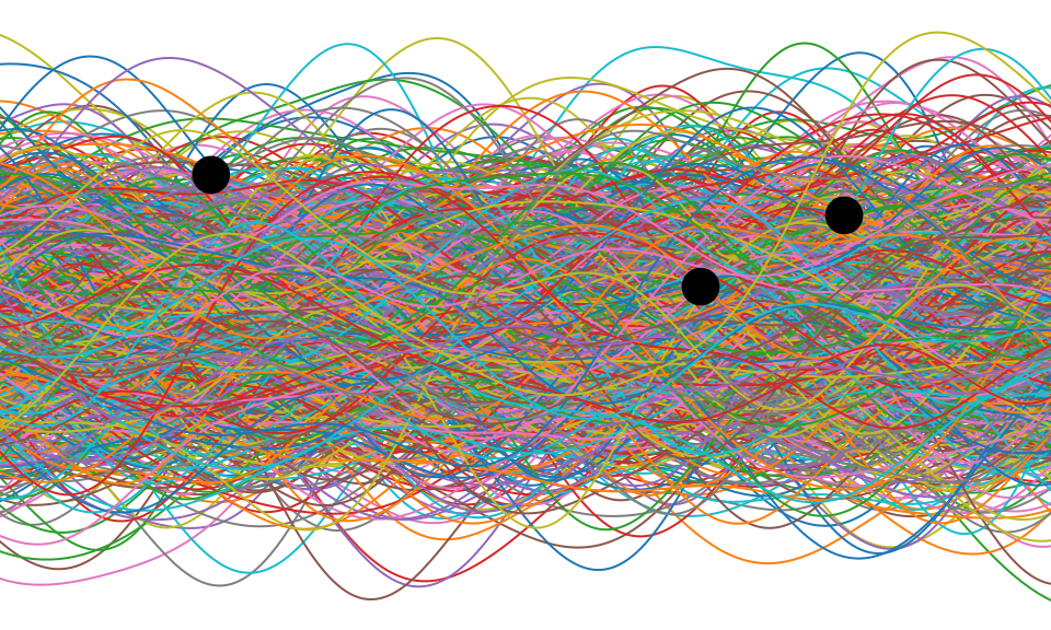
Prediction with Correlated Gaussians

• Prediction of \(f_2\) from \(f_1\) requires conditional density.
• Conditional density is also Gaussian. \[ p(f_2|f_1) = \mathcal{N}\left(f_2|\frac{k_{1, 2}}{k_{1, 1}}f_1, k_{2, 2} - \frac{k_{1,2}^2}{k_{1,1}}\right) \] where covariance of joint density is given by \[ \mathbf{K}= \begin{bmatrix} k_{1, 1} & k_{1, 2}\\ k_{2, 1} & k_{2, 2}.\end{bmatrix} \]

Joint Density of \(f_1\) and \(f_8\)

Prediction of \(f_{8}\) from \(f_{1}\)

❮ ❯

Details

• The single contour of the Gaussian density represents the joint distribution, \(p(f_1, f_8)\)

Prediction with Correlated Gaussians

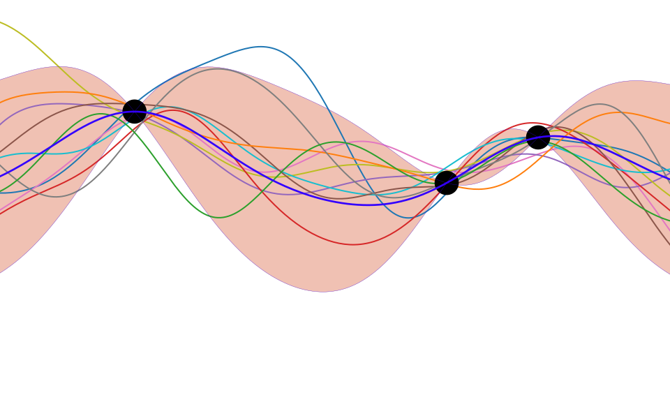
• Prediction of \(\mathbf{ f}_*\) from \(\mathbf{ f}\) requires multivariate conditional density.

• Multivariate conditional density is also Gaussian. \[ p(\mathbf{ f}_*|\mathbf{ f}) = {\mathcal{N}\left(\mathbf{ f}_*|\mathbf{K}_{*,\mathbf{ f}}\mathbf{K}_{\mathbf{ f},\mathbf{ f}}^{-1}\mathbf{ f},\mathbf{K}_{*,*}-\mathbf{K}_{*,\mathbf{ f}} \mathbf{K}_{\mathbf{ f},\mathbf{ f}}^{-1}\mathbf{K}_{\mathbf{ f},*}\right)} \]

• Here covariance of joint density is given by \[ \mathbf{K}= \begin{bmatrix} \mathbf{K}_{\mathbf{ f}, \mathbf{ f}} & \mathbf{K}_{*, \mathbf{ f}}\\ \mathbf{K}_{\mathbf{ f}, *} & \mathbf{K}_{*, *}\end{bmatrix} \]

Prediction with Correlated Gaussians

• Prediction of \(\mathbf{ f}_*\) from \(\mathbf{ f}\) requires multivariate conditional density.

• Multivariate conditional density is also Gaussian. \[ p(\mathbf{ f}_*|\mathbf{ f}) = {\mathcal{N}\left(\mathbf{ f}_*|\boldsymbol{ \mu},\boldsymbol{ \Sigma}\right)} \] \[ \boldsymbol{ \mu}= \mathbf{K}_{*,\mathbf{ f}}\mathbf{K}_{\mathbf{ f},\mathbf{ f}}^{-1}\mathbf{ f} \] \[ \boldsymbol{ \Sigma}= \mathbf{K}_{*,*}-\mathbf{K}_{*,\mathbf{ f}} \mathbf{K}_{\mathbf{ f},\mathbf{ f}}^{-1}\mathbf{K}_{\mathbf{ f},*} \]

• Here covariance of joint density is given by \[ \mathbf{K}= \begin{bmatrix} \mathbf{K}_{\mathbf{ f}, \mathbf{ f}} & \mathbf{K}_{*, \mathbf{ f}}\\ \mathbf{K}_{\mathbf{ f}, *} & \mathbf{K}_{*, *}\end{bmatrix} \]

Where Did This Covariance Matrix Come From?

\[ k(\mathbf{ x}, \mathbf{ x}^\prime) = \alpha \exp\left(-\frac{\left\Vert \mathbf{ x}- \mathbf{ x}^\prime\right\Vert^2_2}{2\ell^2}\right)\]

Computing Covariance

❮ ❯

Computing Covariance

❮ ❯

Computing Covariance

❮ ❯

Polynomial Covariance

Degenerate Covariance Functions

RBF Basis Functions

\[ \phi_k(x) = \exp\left(-\frac{\left\Vert x-\mu_k \right\Vert_2^{2}}{\ell^{2}}\right). \]

\[ \boldsymbol{ \mu}= \begin{bmatrix} -1 \\ 0 \\ 1\end{bmatrix}, \]

\[ k\left(\mathbf{ x},\mathbf{ x}^{\prime}\right)=\alpha\boldsymbol{ \phi}(\mathbf{ x})^\top \boldsymbol{ \phi}(\mathbf{ x}^\prime). \]

Basis Function Covariance

Selecting Number and Location of Basis

• Need to choose
  1. location of centers
  2. number of basis functions Restrict analysis to 1-D input, \(x\).
• Consider uniform spacing over a region:

Uniform Basis Functions

• Set each center location to \[\mu_k = a+\Delta\mu\cdot (k-1).\]

• Specify the basis functions in terms of their indices, \[\begin{aligned} k\left(x_i,x_j\right) = &\alpha^\prime\Delta\mu\sum_{k=1}^{m} \exp\Bigg( -\frac{x_i^2 + x_j^2}{2\ell^2}\\ & - \frac{2\left(a+\Delta\mu\cdot (k-1)\right) \left(x_i+x_j\right) + 2\left(a+\Delta\mu\cdot (k-1)\right)^2}{2\ell^2} \Bigg) \end{aligned}\]

where we’ve scaled variance of process by \(\Delta\mu\).

Infinite Basis Functions

• Take \[ \mu_1=a \ \text{and}\ \mu_m=b \ \text{so}\ b= a+ \Delta\mu\cdot(m-1) \]

• This implies \[ b-a = \Delta\mu(m-1) \] and therefore \[ m= \frac{b-a}{\Delta \mu} + 1 \]

• Take limit as \(\Delta\mu\rightarrow 0\) so \(m\rightarrow \infty\) where we have used \(a + k\cdot\Delta\mu\rightarrow \mu\).

Result

• Performing the integration leads to \[\begin{aligned} k(x_i,&x_j) = \alpha^\prime \sqrt{\pi\ell^2} \exp\left( -\frac{\left(x_i-x_j\right)^2}{4\ell^2}\right)\\ &\times \frac{1}{2}\left[\text{erf}\left(\frac{\left(b - \frac{1}{2}\left(x_i + x_j\right)\right)}{\ell} \right)- \text{erf}\left(\frac{\left(a - \frac{1}{2}\left(x_i + x_j\right)\right)}{\ell} \right)\right], \end{aligned}\]
• Now take limit as \(a\rightarrow -\infty\) and \(b\rightarrow \infty\) \[k\left(x_i,x_j\right) = \alpha\exp\left( -\frac{\left(x_i-x_j\right)^2}{4\ell^2}\right).\] where \(\alpha=\alpha^\prime \sqrt{\pi\ell^2}\).

Infinite Feature Space

• An RBF model with infinite basis functions is a Gaussian process.
• The covariance function is given by the  covariance function. \[k\left(x_i,x_j\right) = \alpha \exp\left( -\frac{\left(x_i-x_j\right)^2}{4\ell^2}\right).\]

Infinite Feature Space

• An RBF model with infinite basis functions is a Gaussian process.
• The covariance function is the exponentiated quadratic (squared exponential).
• Note: The functional form for the covariance function and basis functions are similar.
  • this is a special case,
  • in general they are very different