Week 1: Uncertainty and Modelling

[Powerpoint][jupyter][google colab][reveal]

Neil D. Lawrence

Abstract:

In this talk we motivate the representation of uncertainty through probability distributions we review Laplace’s approach to understanding uncertainty and how uncertainty in functions can be represented through a multivariate Gaussian density.

Figure: A key reference for Gaussian process models remains the excellent book “Gaussian Processes for Machine Learning” (Rasmussen and Williams (2006)). The book is also freely available online.

Rasmussen and Williams (2006) is still one of the most important references on Gaussian process models. It is available freely online.

What is Machine Learning?

What is machine learning? At its most basic level machine learning is a combination of

\[\text{data} + \text{model} \stackrel{\text{compute}}{\rightarrow} \text{prediction}\]

where data is our observations. They can be actively or passively acquired (meta-data). The model contains our assumptions, based on previous experience. That experience can be other data, it can come from transfer learning, or it can merely be our beliefs about the regularities of the universe. In humans our models include our inductive biases. The prediction is an action to be taken or a categorization or a quality score. The reason that machine learning has become a mainstay of artificial intelligence is the importance of predictions in artificial intelligence. The data and the model are combined through computation.

In practice we normally perform machine learning using two functions. To combine data with a model we typically make use of:

a prediction function it is used to make the predictions. It includes our beliefs about the regularities of the universe, our assumptions about how the world works, e.g., smoothness, spatial similarities, temporal similarities.

an objective function it defines the ‘cost’ of misprediction. Typically, it includes knowledge about the world’s generating processes (probabilistic objectives) or the costs we pay for mispredictions (empirical risk minimization).

The combination of data and model through the prediction function and the objective function leads to a learning algorithm. The class of prediction functions and objective functions we can make use of is restricted by the algorithms they lead to. If the prediction function or the objective function are too complex, then it can be difficult to find an appropriate learning algorithm. Much of the academic field of machine learning is the quest for new learning algorithms that allow us to bring different types of models and data together.

A useful reference for state of the art in machine learning is the UK Royal Society Report, Machine Learning: Power and Promise of Computers that Learn by Example.

You can also check my post blog post on What is Machine Learning?.

%pip install gpy

GPy: A Gaussian Process Framework in Python

Gaussian processes are a flexible tool for non-parametric analysis with uncertainty. The GPy software was started in Sheffield to provide a easy to use interface to GPs. One which allowed the user to focus on the modelling rather than the mathematics.

Figure: GPy is a BSD licensed software code base for implementing Gaussian process models in Python. It is designed for teaching and modelling. We welcome contributions which can be made through the GitHub repository https://github.com/SheffieldML/GPy

GPy is a BSD licensed software code base for implementing Gaussian process models in python. This allows GPs to be combined with a wide variety of software libraries.

The software itself is available on GitHub and the team welcomes contributions.

The aim for GPy is to be a probabilistic-style programming language, i.e., you specify the model rather than the algorithm. As well as a large range of covariance functions the software allows for non-Gaussian likelihoods, multivariate outputs, dimensionality reduction and approximations for larger data sets.

The documentation for GPy can be found here.

Olympic Marathon Data

Gold medal times for Olympic Marathon since 1896. Marathons before 1924 didn’t have a standardized distance. Present results using pace per km. In 1904 Marathon was badly organized leading to very slow times.

Image from Wikimedia Commons http://bit.ly/16kMKHQ

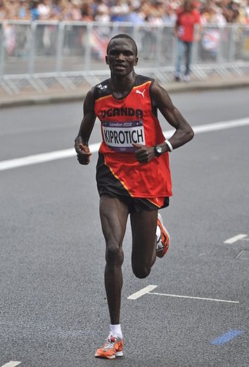
The first thing we will do is load a standard data set for regression modelling. The data consists of the pace of Olympic Gold Medal Marathon winners for the Olympics from 1896 to present. Let’s load in the data and plot.

%pip install pods

import numpy as np
import pods

data = pods.datasets.olympic_marathon_men()
x = data['X']
y = data['Y']

offset = y.mean()
scale = np.sqrt(y.var())
yhat = (y - offset)/scale

Figure: Olympic marathon pace times since 1896.

Things to notice about the data include the outlier in 1904, in that year the Olympics was in St Louis, USA. Organizational problems and challenges with dust kicked up by the cars following the race meant that participants got lost, and only very few participants completed. More recent years see more consistently quick marathons.

Overdetermined System

The challenge with a linear model is that it has two unknowns, \(m\), and \(c\). Observing data allows us to write down a system of simultaneous linear equations. So, for example if we observe two data points, the first with the input value, \(x_1 = 1\) and the output value, \(y_1 =3\) and a second data point, \(x= 3\), \(y=1\), then we can write two simultaneous linear equations of the form.

point 1: \(x= 1\), \(y=3\) \[ 3 = m + c \] point 2: \(x= 3\), \(y=1\) \[ 1 = 3m + c \]

The solution to these two simultaneous equations can be represented graphically as

Figure: The solution of two linear equations represented as the fit of a straight line through two data

The challenge comes when a third data point is observed, and it doesn’t fit on the straight line.

point 3: \(x= 2\), \(y=2.5\) \[ 2.5 = 2m + c \]

Figure: A third observation of data is inconsistent with the solution dictated by the first two observations

Now there are three candidate lines, each consistent with our data.

Figure: Three solutions to the problem, each consistent with two points of the three observations

This is known as an overdetermined system because there are more data than we need to determine our parameters. The problem arises because the model is a simplification of the real world, and the data we observe is therefore inconsistent with our model.

Pierre-Simon Laplace

The solution was proposed by Pierre-Simon Laplace. His idea was to accept that the model was an incomplete representation of the real world, and the way it was incomplete is unknown. His idea was that such unknowns could be dealt with through probability.

Pierre-Simon Laplace

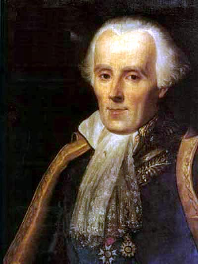
Figure: Pierre-Simon Laplace 1749-1827.

Famously, Laplace considered the idea of a deterministic Universe, one in which the model is known, or as the below translation refers to it, “an intelligence which could comprehend all the forces by which nature is animated”. He speculates on an “intelligence” that can submit this vast data to analysis and propsoses that such an entity would be able to predict the future.

Given for one instant an intelligence which could comprehend all the forces by which nature is animated and the respective situation of the beings who compose it—an intelligence sufficiently vast to submit these data to analysis—it would embrace in the same formulate the movements of the greatest bodies of the universe and those of the lightest atom; for it, nothing would be uncertain and the future, as the past, would be present in its eyes.

This notion is known as Laplace’s demon or Laplace’s superman.

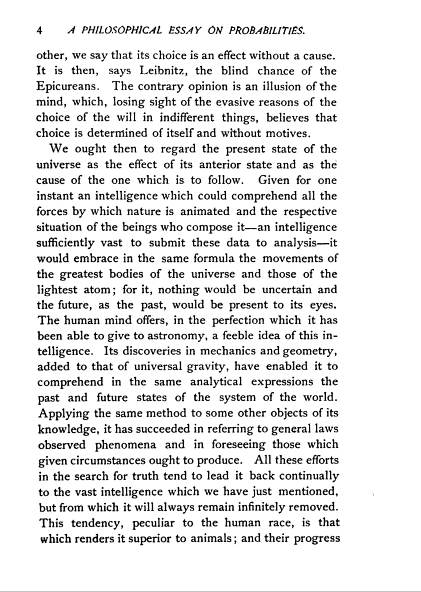
Figure: Laplace’s determinsim in English translation.

Laplace’s Gremlin

Unfortunately, most analyses of his ideas stop at that point, whereas his real point is that such a notion is unreachable. Not so much superman as strawman. Just three pages later in the “Philosophical Essay on Probabilities” (Laplace, 1814), Laplace goes on to observe:

The curve described by a simple molecule of air or vapor is regulated in a manner just as certain as the planetary orbits; the only difference between them is that which comes from our ignorance.

Probability is relative, in part to this ignorance, in part to our knowledge.

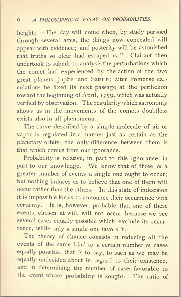
Figure: To Laplace, determinism is a strawman. Ignorance of mechanism and data leads to uncertainty which should be dealt with through probability.

In other words, we can never make use of the idealistic deterministic Universe due to our ignorance about the world, Laplace’s suggestion, and focus in this essay is that we turn to probability to deal with this uncertainty. This is also our inspiration for using probability in machine learning. This is the true message of Laplace’s essay, not determinism, but the gremlin of uncertainty that emerges from our ignorance.

The “forces by which nature is animated” is our model, the “situation of beings that compose it” is our data and the “intelligence sufficiently vast enough to submit these data to analysis” is our compute. The fly in the ointment is our ignorance about these aspects. And probability is the tool we use to incorporate this ignorance leading to uncertainty or doubt in our predictions.

Latent Variables

Laplace’s concept was that the reason that the data doesn’t match up to the model is because of unconsidered factors, and that these might be well represented through probability densities. He tackles the challenge of the unknown factors by adding a variable, \(\epsilon\), that represents the unknown. In modern parlance we would call this a latent variable. But in the context Laplace uses it, the variable is so common that it has other names such as a “slack” variable or the noise in the system.

point 1: \(x= 1\), \(y=3\) [ 3 = m + c + _1 ] point 2: \(x= 3\), \(y=1\) [ 1 = 3m + c + _2 ] point 3: \(x= 2\), \(y=2.5\) [ 2.5 = 2m + c + _3 ]

Laplace’s trick has converted the overdetermined system into an underdetermined system. He has now added three variables, \(\{\epsilon_i\}_{i=1}^3\), which represent the unknown corruptions of the real world. Laplace’s idea is that we should represent that unknown corruption with a probability distribution.

A Probabilistic Process

However, it was left to an admirer of Laplace to develop a practical probability density for that purpose. It was Carl Friedrich Gauss who suggested that the Gaussian density (which at the time was unnamed!) should be used to represent this error.

The result is a noisy function, a function which has a deterministic part, and a stochastic part. This type of function is sometimes known as a probabilistic or stochastic process, to distinguish it from a deterministic process.

The Gaussian Density

The Gaussian density is perhaps the most commonly used probability density. It is defined by a mean, \(\mu\), and a variance, \(\sigma^2\). The variance is taken to be the square of the standard deviation, \(\sigma\).

\[\begin{align} p(y| \mu, \sigma^2) & = \frac{1}{\sqrt{2\pi\sigma^2}}\exp\left(-\frac{(y- \mu)^2}{2\sigma^2}\right)\\& \buildrel\triangle\over = \mathcal{N}\left(y|\mu,\sigma^2\right) \end{align}\]

Figure: The Gaussian PDF with \({\mu}=1.7\) and variance \({\sigma}^2=0.0225\). Mean shown as red line. It could represent the heights of a population of students.

Two Important Gaussian Properties

The Gaussian density has many important properties, but for the moment we’ll review two of them.

Sum of Gaussians

If we assume that a variable, \(y_i\), is sampled from a Gaussian density,

\[y_i \sim \mathcal{N}\left(\mu_i,\sigma_i^2\right)\]

Then we can show that the sum of a set of variables, each drawn independently from such a density is also distributed as Gaussian. The mean of the resulting density is the sum of the means, and the variance is the sum of the variances,

\[ \sum_{i=1}^{n} y_i \sim \mathcal{N}\left(\sum_{i=1}^n\mu_i,\sum_{i=1}^n\sigma_i^2\right) \]

Since we are very familiar with the Gaussian density and its properties, it is not immediately apparent how unusual this is. Most random variables, when you add them together, change the family of density they are drawn from. For example, the Gaussian is exceptional in this regard. Indeed, other random variables, if they are independently drawn and summed together tend to a Gaussian density. That is the central limit theorem which is a major justification for the use of a Gaussian density.

Scaling a Gaussian

Less unusual is the scaling property of a Gaussian density. If a variable, \(y\), is sampled from a Gaussian density,

\[y\sim \mathcal{N}\left(\mu,\sigma^2\right)\] and we choose to scale that variable by a deterministic value, \(w\), then the scaled variable is distributed as

\[wy\sim \mathcal{N}\left(w\mu,w^2 \sigma^2\right).\] Unlike the summing properties, where adding two or more random variables independently sampled from a family of densitites typically brings the summed variable outside that family, scaling many densities leaves the distribution of that variable in the same family of densities. Indeed, many densities include a scale parameter (e.g. the Gamma density) which is purely for this purpose. In the Gaussian the standard deviation, \(\sigma\), is the scale parameter. To see why this makes sense, let’s consider, \[z \sim \mathcal{N}\left(0,1\right),\] then if we scale by \(\sigma\) so we have, \(y=\sigma z\), we can write, \[y=\sigma z \sim \mathcal{N}\left(0,\sigma^2\right)\]

Regression Examples

Regression involves predicting a real value, \(y_i\), given an input vector, \(\mathbf{ x}_i\). For example, the Tecator data involves predicting the quality of meat given spectral measurements. Or in radiocarbon dating, the C14 calibration curve maps from radiocarbon age to age measured through a back-trace of tree rings. Regression has also been used to predict the quality of board game moves given expert rated training data.

Underdetermined System

What about the situation where you have more parameters than data in your simultaneous equation? This is known as an underdetermined system. In fact, this set up is in some sense easier to solve, because we don’t need to think about introducing a slack variable (although it might make a lot of sense from a modelling perspective to do so).

The way Laplace proposed resolving an overdetermined system, was to introduce slack variables, \(\epsilon_i\), which needed to be estimated for each point. The slack variable represented the difference between our actual prediction and the true observation. This is known as the residual. By introducing the slack variable, we now have an additional \(n\) variables to estimate, one for each data point, \(\{\epsilon_i\}\). This turns the overdetermined system into an underdetermined system. Introduction of \(n\) variables, plus the original \(m\) and \(c\) gives us \(n+2\) parameters to be estimated from \(n\) observations, which makes the system underdetermined. However, we then made a probabilistic assumption about the slack variables, we assumed that the slack variables were distributed according to a probability density. And for the moment we have been assuming that density was the Gaussian, \[\epsilon_i \sim \mathcal{N}\left(0,\sigma^2\right),\] with zero mean and variance \(\sigma^2\).

The follow up question is whether we can do the same thing with the parameters. If we have two parameters and only one unknown, can we place a probability distribution over the parameters as we did with the slack variables? The answer is yes.

Underdetermined System

Figure: An underdetermined system can be fit by considering uncertainty. Multiple solutions are consistent with one specified point.

Classically, there are two types of uncertainty that we consider. The first is known as aleatoric uncertainty. This is uncertainty we couldn’t resolve even if we wanted to. An example, would be the result of a football match before it’s played, or where a sheet of paper lands on the floor.

The second is known as epistemic uncertainty. This is uncertainty that we could, in principle, resolve. We just haven’t yet made the observation. For example, the result of a football match after it is played, or the color of socks that a lecturer is wearing.

Note, that there isn’t a clean difference between the two. It is arguable, that if we knew enough about a football match, or the physics of a falling sheet of paper then we might be able to resolve the uncertainty. The reason we can’t is because chaotic behaviour means that a very small change in any of the initial conditions we would need to resolve can have a large change in downstream effects. By this argument, the only truly aleatoric uncertainty might be quantum uncertainty. However, in practice the distinction is often applied.

In classical statistics, the frequentist approach only treats aleatoric uncertainty with probability. The key philosophical difference in the Bayesian approach is to treat any unknowns through probability. This approach was formally justified seperately by Cox (1946) and Finetti (1937).

The term Bayesian was a mocking term promoted by Fisher, it comes from the use, by Bayes, of a billiard table formulation to justify the Bernoulli distribution. Bayes considers a ball landing uniform at random between two sides of a billiard table. He then considers the outcome of the Bernoulli as being whether a second ball comes to rest to the right or left of the original. In this way, the parameter of his Bernoulli distribution is a stochastic variable (the uncertainty in the parameter is aleatoric). In contrast, when Bernoulli formulates the distribution he considers a bag of red and black balls. The parameter of his Bernoulli is the ratio of red balls to total balls, a deterministic variable.

Note how this relates to Laplace’s demon. Laplace describes the deterministic universe (“… for it nothing would be uncertain and the future, as the past, would be present in its eyes”), but acknowledges the impossibility of achieving this in practice, (” … the curve described by a simple molecule of air or vapor is regulated in a manner just as certain as the planetary orbits; the only difference between them is that which comes from our ignorance. Probability is relative in part to this ignorance, in part to our knowledge …)

Prior Distribution

The tradition in Bayesian inference is to place a probability density over the parameters of interest in your model. This choice is made regardless of whether you generally believe those parameters to be stochastic or deterministic in origin. In other words, to a Bayesian, the modelling treatment does not differentiate between epistemic and aleatoric uncertainty. For linear regression we could consider the following Gaussian prior on the intercept parameter, \[c \sim \mathcal{N}\left(0,\alpha_1\right)\] where \(\alpha_1\) is the variance of the prior distribution, its mean being zero.

Posterior Distribution

The prior distribution is combined with the likelihood of the data given the parameters \(p(y|c)\) to give the posterior via Bayes’ rule, \[ p(c|y) = \frac{p(y|c)p(c)}{p(y)} \] where \(p(y)\) is the marginal probability of the data, obtained through integration over the joint density, \(p(y, c)=p(y|c)p(c)\). Overall the equation can be summarized as, \[ \text{posterior} = \frac{\text{likelihood}\times \text{prior}}{\text{marginal likelihood}}. \]

Figure: Combining a Gaussian likelihood with a Gaussian prior to form a Gaussian posterior

Another way of seeing what’s going on is to note that the numerator of Bayes’ rule merely multiplies the likelihood by the prior. The denominator, is not a function of \(c\). So the functional form is entirely determined by the multiplication of prior and likelihood. This has the effect of ensuring that the posterior only has probability mass in regions where both the prior and the likelihood have probability mass.

The marginal likelihood, \(p(y)\), operates to ensure that the distribution is normalised.

For the Gaussian case, the normalisation of the posterior can be performed analytically. This is because both the prior and the likelihood have the form of an exponentiated quadratic, \[ \exp(a^2)\exp(b^2) = \exp(a^2 + b^2), \] and the properties of the exponential mean that the product of two exponentiated quadratics is also an exponentiated quadratic. That implies that the posterior is also Gaussian, because a normalized exponentiated quadratic is a Gaussian distribution.¹

For general Bayesian inference, over more than one parameter, we need multivariate priors. For example, consider the multivariate linear regression where an observation, \(y_i\) is related to a vector of features, \(\mathbf{ x}_{i, :}\), through a vector of parameters, \(\mathbf{ w}\), \[y_i = \sum_j w_j x_{i, j} + \epsilon_i,\] or in vector notation, \[y_i = \mathbf{ w}^\top \mathbf{ x}_{i, :} + \epsilon_i.\] Here we’ve dropped the intercpet for convenience, it can be reintroduced by augmenting the feature vector, \(\mathbf{ x}_{i, :}\), with a constant valued feature.

This motivates the need for a multivariate Gaussian density.

Multivariate Regression Likelihood

• Noise corrupted data point \[y_i = \mathbf{ w}^\top \mathbf{ x}_{i, :} + {\epsilon}_i\]

. . .

• Multivariate regression likelihood: \[p(\mathbf{ y}| \mathbf{X}, \mathbf{ w}) = \frac{1}{\left(2\pi {\sigma}^2\right)^{n/2}} \exp\left(-\frac{1}{2{\sigma}^2}\sum_{i=1}^{n}\left(y_i - \mathbf{ w}^\top \mathbf{ x}_{i, :}\right)^2\right)\]

. . .

• Now use a multivariate Gaussian prior: \[p(\mathbf{ w}) = \frac{1}{\left(2\pi \alpha\right)^\frac{p}{2}} \exp \left(-\frac{1}{2\alpha} \mathbf{ w}^\top \mathbf{ w}\right)\]

Thanks!

For more information on these subjects and more you might want to check the following resources.

• twitter: @lawrennd
• podcast: The Talking Machines
• newspaper: Guardian Profile Page
• blog: http://inverseprobability.com

References