Uncertainty and Modelling

Rasmussen and Williams (2006)

What is Machine Learning?

\[ \text{data} + \text{model} \stackrel{\text{compute}}{\rightarrow} \text{prediction}\]

data : observations, could be actively or passively acquired (meta-data).

model : assumptions, based on previous experience (other data! transfer learning etc), or beliefs about the regularities of the universe. Inductive bias.

prediction : an action to be taken or a categorization or a quality score.

Royal Society Report: Machine Learning: Power and Promise of Computers that Learn by Example

What is Machine Learning?

\[\text{data} + \text{model} \stackrel{\text{compute}}{\rightarrow} \text{prediction}\]

To combine data with a model need:
a prediction function \(f(\cdot)\) includes our beliefs about the regularities of the universe
an objective function \(E(\cdot)\) defines the cost of misprediction.

GPy: A Gaussian Process Framework in Python

https://github.com/SheffieldML/GPy

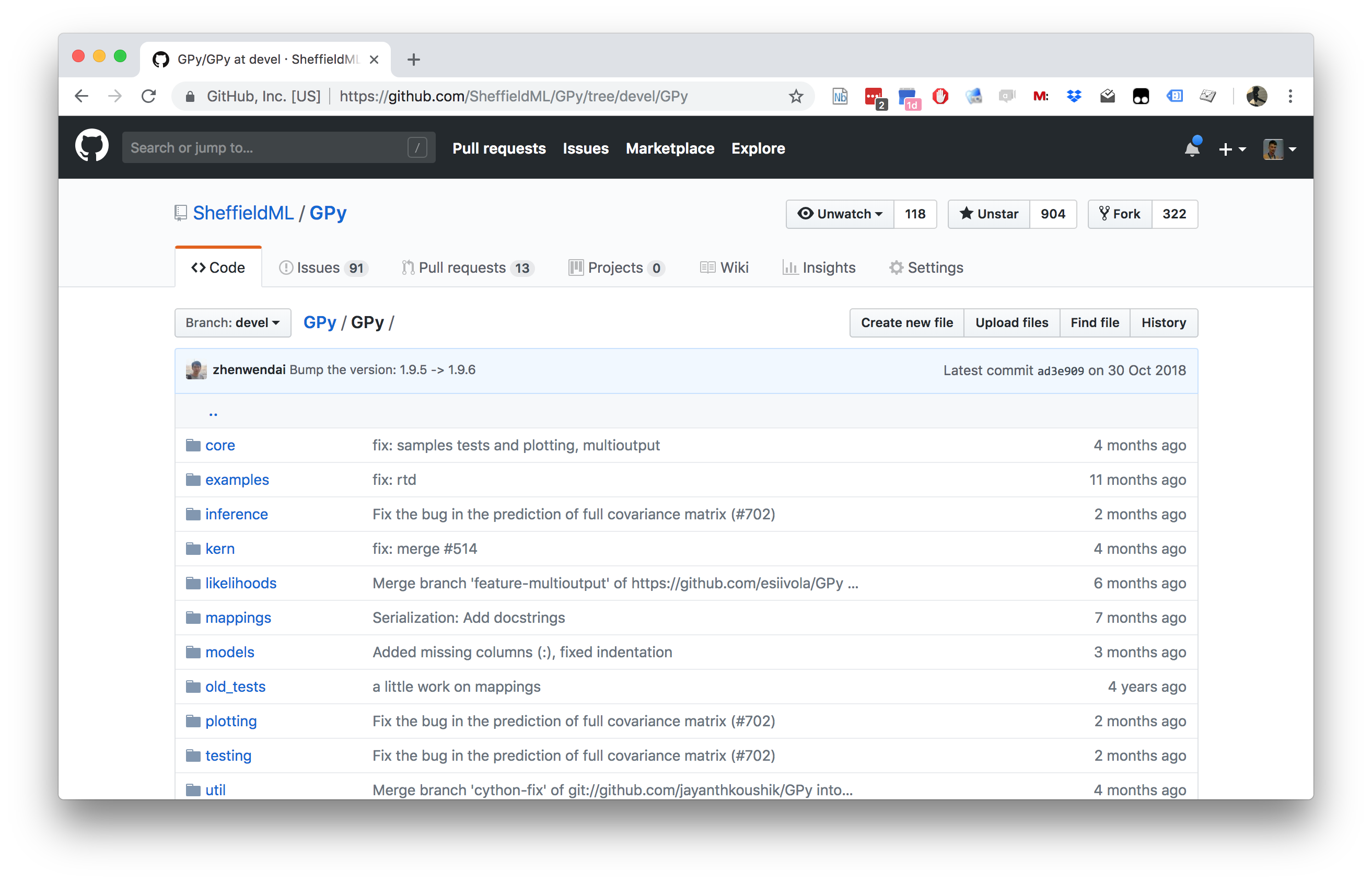
GPy: A Gaussian Process Framework in Python

BSD Licensed software base.
Wide availability of libraries, ‘modern’ scripting language.
Allows us to set projects to undergraduates in Comp Sci that use GPs.
Available through GitHub https://github.com/SheffieldML/GPy
Reproducible Research with Jupyter Notebook.

Features

Probabilistic-style programming (specify the model, not the algorithm).
Non-Gaussian likelihoods.
Multivariate outputs.
Dimensionality reduction.
Approximations for large data sets.

Olympic Marathon Data

Gold medal times for Olympic Marathon since 1896.
Marathons before 1924 didn’t have a standardized distance.
Present results using pace per km.
In 1904 Marathon was badly organized leading to very slow times.

Image from Wikimedia Commons http://bit.ly/16kMKHQ

Olympic Marathon Data

Overdetermined System

\(y= mx+ c\)

point 1: \(x= 1\), \(y=3\) \[ 3 = m + c \]

point 2: \(x= 3\), \(y=1\) \[ 1 = 3m + c \]

point 3: \(x= 2\), \(y=2.5\) \[ 2.5 = 2m + c \]

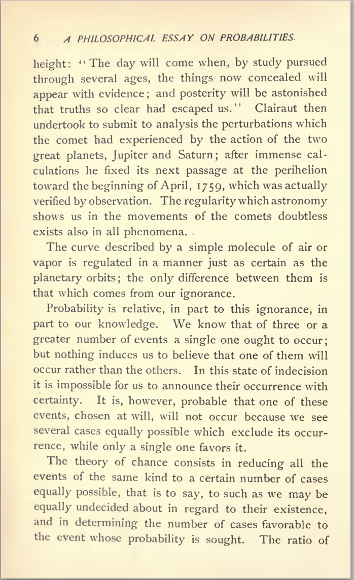
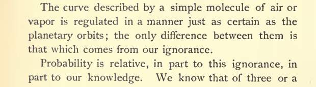
Pierre-Simon Laplace

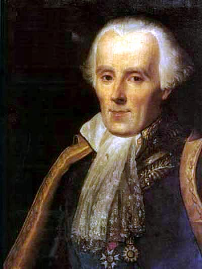
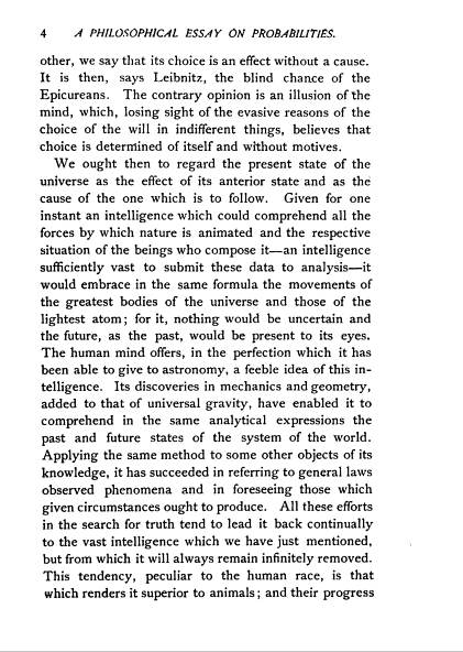
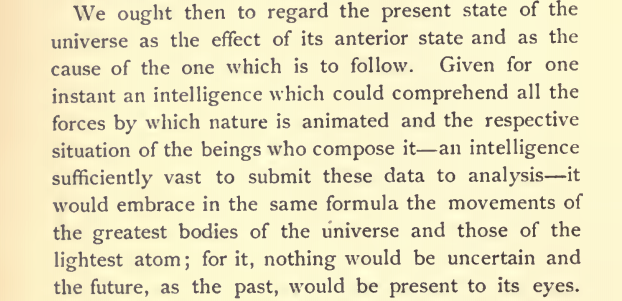
Laplace’s Gremlin

Latent Variables

\(y= mx+ c + \epsilon\)

point 1: \(x= 1\), \(y=3\) [ 3 = m + c + _1 ]

point 2: \(x= 3\), \(y=1\) [ 1 = 3m + c + _2 ]

point 3: \(x= 2\), \(y=2.5\) [ 2.5 = 2m + c + _3 ]

A Probabilistic Process

Set the mean of Gaussian to be a function. \[ p\left(y_i|x_i\right)=\frac{1}{\sqrt{2\pi\sigma^2}}\exp \left(-\frac{\left(y_i-f\left(x_i\right)\right)^{2}}{2\sigma^2}\right). \]

This gives us a ‘noisy function’.

This is known as a stochastic process.

The Gaussian Density

Perhaps the most common probability density.

\[\begin{align} p(y| \mu, \sigma^2) & = \frac{1}{\sqrt{2\pi\sigma^2}}\exp\left(-\frac{(y- \mu)^2}{2\sigma^2}\right)\\& \buildrel\triangle\over = \mathcal{N}\left(y|\mu,\sigma^2\right) \end{align}\]

Gaussian Density

\[ \mathcal{N}\left(y|\mu,\sigma^2\right) = \frac{1}{\sqrt{2\pi\sigma^2}} \exp\left(-\frac{(y-\mu)^2}{2\sigma^2}\right) \]

\(\sigma^2\) is the variance of the density and \(\mu\) is the mean.

Two Important Gaussian Properties

Sum of Gaussians

Sum of Gaussian variables is also Gaussian.

\[y_i \sim \mathcal{N}\left(\mu_i,\sigma_i^2\right)\]

And the sum is distributed as

\[ \sum_{i=1}^{n} y_i \sim \mathcal{N}\left(\sum_{i=1}^n\mu_i,\sum_{i=1}^n\sigma_i^2\right) \]

(Aside: As sum increases, sum of non-Gaussian, finite variance variables is also Gaussian because of central limit theorem.)

Scaling a Gaussian

Scaling a Gaussian leads to a Gaussian.

\[y\sim \mathcal{N}\left(\mu,\sigma^2\right)\]

And the scaled variable is distributed as

\[wy\sim \mathcal{N}\left(w\mu,w^2 \sigma^2\right).\]

Regression Examples

Predict a real value, \(y_i\) given some inputs \(\mathbf{ x}_i\).
Predict quality of meat given spectral measurements (Tecator data).
Radiocarbon dating, the C14 calibration curve: predict age given quantity of C14 isotope.
Predict quality of different Go or Backgammon moves given expert rated training data.

Underdetermined System

What about two unknowns and one observation? \[y_1 = mx_1 + c\]

Can compute \(m\) given \(c\). \[m = \frac{y_1 - c}{x}\]

Underdetermined System

Overdetermined System

With two unknowns and two observations: \[ \begin{aligned} y_1 = & mx_1 + c\\ y_2 = & mx_2 + c \end{aligned} \]
Additional observation leads to overdetermined system. \[y_3 = mx_3 + c\]

Overdetermined System

This problem is solved through a noise model \(\epsilon\sim \mathcal{N}\left(0,\sigma^2\right)\) \[\begin{aligned} y_1 = mx_1 + c + \epsilon_1\\ y_2 = mx_2 + c + \epsilon_2\\ y_3 = mx_3 + c + \epsilon_3 \end{aligned}\]

Noise Models

We aren’t modeling entire system.
Noise model gives mismatch between model and data.
Gaussian model justified by appeal to central limit theorem.
Other models also possible (Student-\(t\) for heavy tails).
Maximum likelihood with Gaussian noise leads to least squares.

Probability for Under- and Overdetermined

To deal with overdetermined introduced probability distribution for ‘variable’, \({\epsilon}_i\).

For underdetermined system introduced probability distribution for ‘parameter’, \(c\).

This is known as a Bayesian treatment.

Different Types of Uncertainty

The first type of uncertainty we are assuming is aleatoric uncertainty.
The second type of uncertainty we are assuming is epistemic uncertainty.

Aleatoric Uncertainty

This is uncertainty we couldn’t know even if we wanted to. e.g. the result of a football match before it’s played.
Where a sheet of paper might land on the floor.

Epistemic Uncertainty

This is uncertainty we could in principle know the answer too. We just haven’t observed enough yet, e.g. the result of a football match after it’s played.
What colour socks your lecturer is wearing.

Bayesian Regression

Prior Distribution

Bayesian inference requires a prior on the parameters.
The prior represents your belief before you see the data of the likely value of the parameters.
For linear regression, consider a Gaussian prior on the intercept:

\[c \sim \mathcal{N}\left(0,\alpha_1\right)\]

Posterior Distribution

Posterior distribution is found by combining the prior with the likelihood.
Posterior distribution is your belief after you see the data of the likely value of the parameters.
The posterior is found through Bayes’ Rule \[ p(c|y) = \frac{p(y|c)p(c)}{p(y)} \]

\[ \text{posterior} = \frac{\text{likelihood}\times \text{prior}}{\text{marginal likelihood}}. \]

Bayes Update

Stages to Derivation of the Posterior

Multiply likelihood by prior
- they are “exponentiated quadratics”, the answer is always also an exponentiated quadratic because \(\exp(a^2)\exp(b^2) = \exp(a^2 + b^2)\).
Complete the square to get the resulting density in the form of a Gaussian.
Recognise the mean and (co)variance of the Gaussian. This is the estimate of the posterior.

Multivariate System

For general Bayesian inference need multivariate priors.

E.g. for multivariate linear regression:

\[y_i = \sum_j w_j x_{i, j} + \epsilon_i,\]

\[y_i = \mathbf{ w}^\top \mathbf{ x}_{i, :} + \epsilon_i.\]

(where we’ve dropped \(c\) for convenience), we need a prior over \(\mathbf{ w}\).

Multivariate System

This motivates a multivariate Gaussian density.

We will use the multivariate Gaussian to put a prior directly on the function (a Gaussian process).

Multivariate Bayesian Regression

Multivariate Regression Likelihood

Noise corrupted data point \[y_i = \mathbf{ w}^\top \mathbf{ x}_{i, :} + {\epsilon}_i\]

Multivariate regression likelihood: \[p(\mathbf{ y}| \mathbf{X}, \mathbf{ w}) = \frac{1}{\left(2\pi {\sigma}^2\right)^{n/2}} \exp\left(-\frac{1}{2{\sigma}^2}\sum_{i=1}^{n}\left(y_i - \mathbf{ w}^\top \mathbf{ x}_{i, :}\right)^2\right)\]

Now use a multivariate Gaussian prior: \[p(\mathbf{ w}) = \frac{1}{\left(2\pi \alpha\right)^\frac{p}{2}} \exp \left(-\frac{1}{2\alpha} \mathbf{ w}^\top \mathbf{ w}\right)\]

Thanks!

References

Rasmussen, C.E., Williams, C.K.I., 2006. Gaussian processes for machine learning. mit, Cambridge, MA.