Gaussian Processes

[jupyter][google colab][reveal][edit]

Venue:Virtual Data Science Nigeria on Friday, Nov 13, 2020 at 15:00 (West Africa Standard Time)

Abstract:

Classical machine learning and statistical approaches to learning, such as neural networks and linear regression, assume a parametric form for functions. Gaussian process models are an alternative approach that assumes a probabilistic prior over functions. This brings benefits, in that uncertainty of function estimation is sustained throughout inference, and some challenges: algorithms for fitting Gaussian processes tend to be more complex than parametric models. In this sessions I will introduce Gaussian processes and explain why sustaining uncertainty is important.

Setup

notutils

This small package is a helper package for various notebook utilities used below.

The software can be installed using

import importlib.util

cmd = install_command('notutils')

%system {cmd}

from the command prompt where you can access your python installation.

The code is also available on GitHub: https://github.com/lawrennd/notutils

Once notutils is installed, it can be imported in the usual manner.

import notutils

pods

In Sheffield we created a suite of software tools for ‘Open Data Science’. Open data science is an approach to sharing code, models and data that should make it easier for companies, health professionals and scientists to gain access to data science techniques.

You can also check this blog post on Open Data Science.

The software can be installed using

cmd = install_command('pods')

%system {cmd}

from the command prompt where you can access your python installation.

The code is also available on GitHub: https://github.com/lawrennd/ods

Once pods is installed, it can be imported in the usual manner.

import pods

mlai

The mlai software is a suite of helper functions for teaching and demonstrating machine learning algorithms. It was first used in the Machine Learning and Adaptive Intelligence course in Sheffield in 2013.

The software can be installed using

cmd = install_command('mlai')

%system {cmd}

from the command prompt where you can access your python installation.

The code is also available on GitHub: https://github.com/lawrennd/mlai

Once mlai is installed, it can be imported in the usual manner.

import mlai
from mlai import plot

Figure: A key reference for Gaussian process models remains the excellent book “Gaussian Processes for Machine Learning” (Rasmussen and Williams (2006)). The book is also freely available online.

Rasmussen and Williams (2006) is still one of the most important references on Gaussian process models. It is available freely online.

A First Course in Machine Learning

Figure: The main course text is “A First Course in Machine Learning” by Rogers and Girolami (2011).

Example: Prediction of Malaria Incidence in Uganda

As an example of using Gaussian process models within the full pipeline from data to decsion, we’ll consider the prediction of Malaria incidence in Uganda. For the purposes of this study malaria reports come in two forms, HMIS reports from health centres and Sentinel data, which is curated by the WHO. There are limited sentinel sites and many HMIS sites.

The work is from Ricardo Andrade Pacheco’s PhD thesis, completed in collaboration with John Quinn and Martin Mubangizi (Andrade-Pacheco et al., 2014; Mubangizi et al., 2014). John and Martin were initally from the AI-DEV group from the University of Makerere in Kampala and more latterly they were based at UN Global Pulse in Kampala. You can see the work summarized on the UN Global Pulse disease outbreaks project site here.

• See UN Global Pulse Disease Outbreaks Site

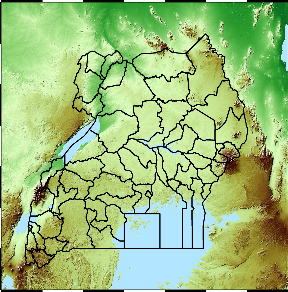
Malaria data is spatial data. Uganda is split into districts, and health reports can be found for each district. This suggests that models such as conditional random fields could be used for spatial modelling, but there are two complexities with this. First of all, occasionally districts split into two. Secondly, sentinel sites are a specific location within a district, such as Nagongera which is a sentinel site based in the Tororo district.

Figure: Ugandan districts. Data SRTM/NASA from https://dds.cr.usgs.gov/srtm/version2_1.

The common standard for collecting health data on the African continent is from the Health management information systems (HMIS). However, this data suffers from missing values (Gething et al., 2006) and diagnosis of diseases like typhoid and malaria may be confounded.

Figure: The Tororo district, where the sentinel site, Nagongera, is located.

World Health Organization Sentinel Surveillance systems are set up “when high-quality data are needed about a particular disease that cannot be obtained through a passive system”. Several sentinel sites give accurate assessment of malaria disease levels in Uganda, including a site in Nagongera.

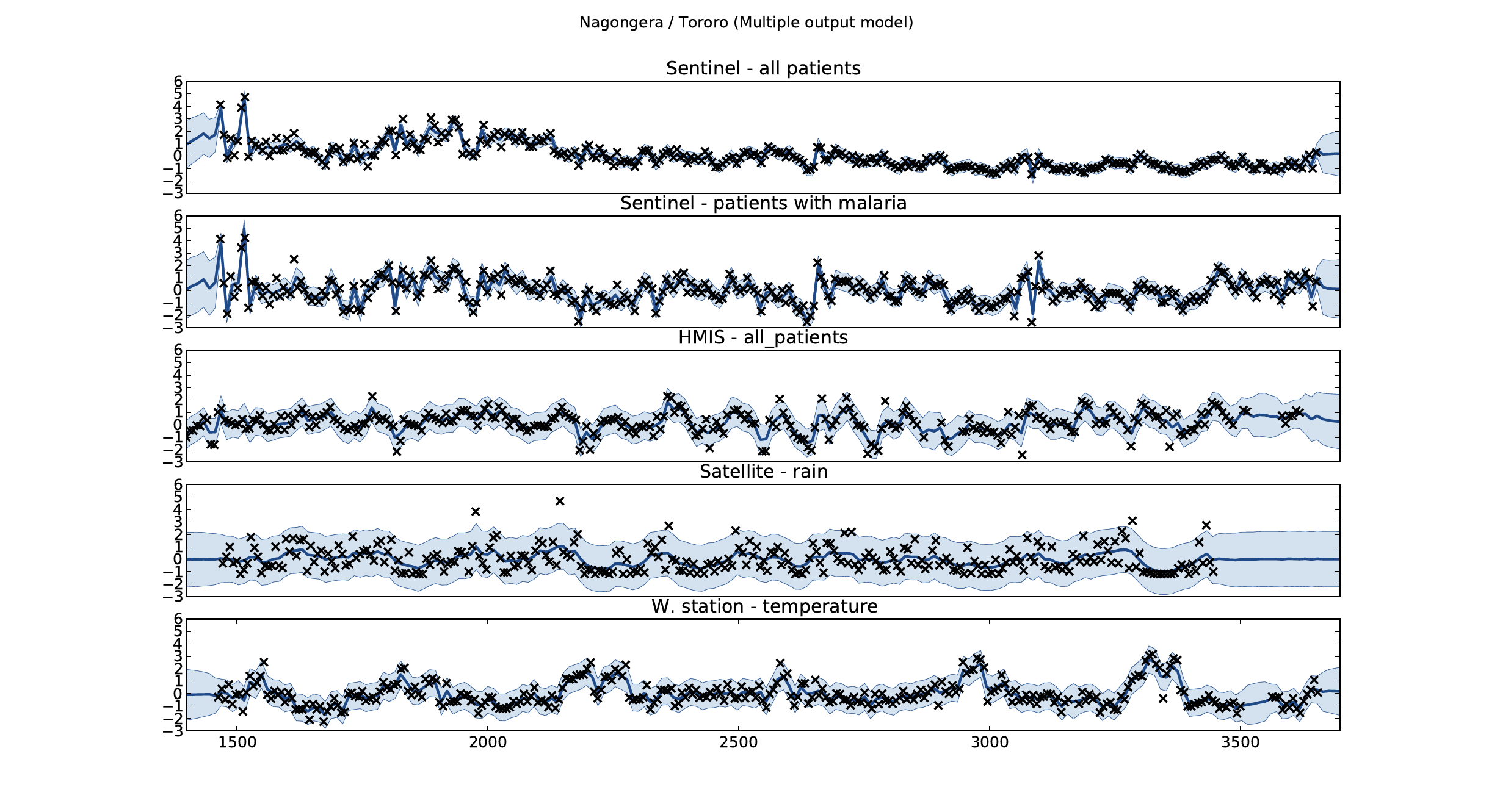
Figure: Sentinel and HMIS data along with rainfall and temperature for the Nagongera sentinel station in the Tororo district.

In collaboration with the AI Research Group at Makerere we chose to investigate whether Gaussian process models could be used to assimilate information from these two different sources of disease informaton. Further, we were interested in whether local information on rainfall and temperature could be used to improve malaria estimates.

The aim of the project was to use WHO Sentinel sites, alongside rainfall and temperature, to improve predictions from HMIS data of levels of malaria.

Figure: The Mubende District.

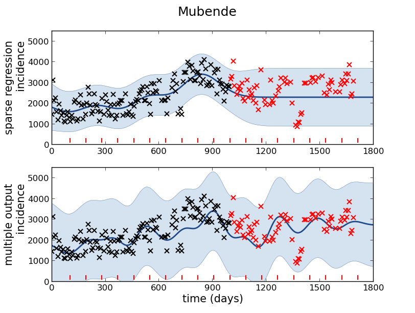
Figure: Prediction of malaria incidence in Mubende.

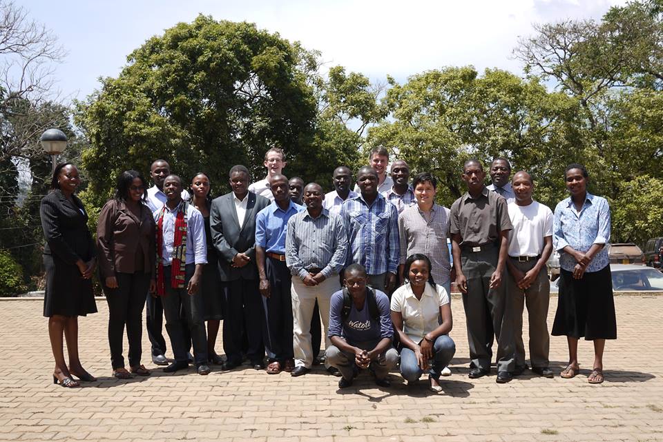
Figure: The project arose out of the Gaussian process summer school held at Makerere in Kampala in 2013. The school led, in turn, to the Data Science Africa initiative.

Early Warning Systems

Figure: The Kabarole district in Uganda.

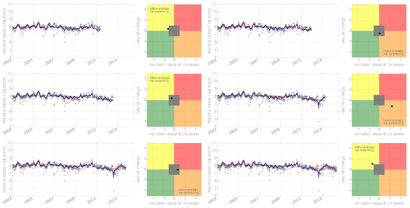
Figure: Estimate of the current disease situation in the Kabarole district over time. Estimate is constructed with a Gaussian process with an additive covariance funciton.

Health monitoring system for the Kabarole district. Here we have fitted the reports with a Gaussian process with an additive covariance function. It has two components, one is a long time scale component (in red above) the other is a short time scale component (in blue).

Monitoring proceeds by considering two aspects of the curve. Is the blue line (the short term report signal) above the red (which represents the long term trend? If so we have higher than expected reports. If this is the case and the gradient is still positive (i.e. reports are going up) we encode this with a red color. If it is the case and the gradient of the blue line is negative (i.e. reports are going down) we encode this with an amber color. Conversely, if the blue line is below the red and decreasing, we color green. On the other hand if it is below red but increasing, we color yellow.

This gives us an early warning system for disease. Red is a bad situation getting worse, amber is bad, but improving. Green is good and getting better and yellow good but degrading.

Finally, there is a gray region which represents when the scale of the effect is small.

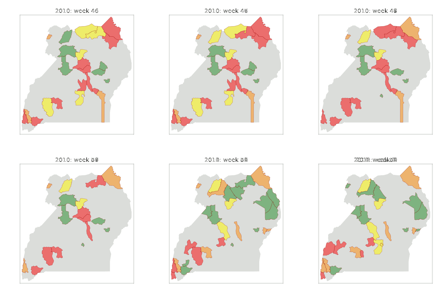
Figure: The map of Ugandan districts with an overview of the Malaria situation in each district.

These colors can now be observed directly on a spatial map of the districts to give an immediate impression of the current status of the disease across the country.

What is Machine Learning?

What is machine learning? At its most basic level machine learning is a combination of

\[\text{data} + \text{model} \stackrel{\text{compute}}{\rightarrow} \text{prediction}\]

where data is our observations. They can be actively or passively acquired (meta-data). The model contains our assumptions, based on previous experience. That experience can be other data, it can come from transfer learning, or it can merely be our beliefs about the regularities of the universe. In humans our models include our inductive biases. The prediction is an action to be taken or a categorization or a quality score. The reason that machine learning has become a mainstay of artificial intelligence is the importance of predictions in artificial intelligence. The data and the model are combined through computation.

In practice we normally perform machine learning using two functions. To combine data with a model we typically make use of:

a prediction function it is used to make the predictions. It includes our beliefs about the regularities of the universe, our assumptions about how the world works, e.g., smoothness, spatial similarities, temporal similarities.

an objective function it defines the ‘cost’ of misprediction. Typically, it includes knowledge about the world’s generating processes (probabilistic objectives) or the costs we pay for mispredictions (empirical risk minimization).

The combination of data and model through the prediction function and the objective function leads to a learning algorithm. The class of prediction functions and objective functions we can make use of is restricted by the algorithms they lead to. If the prediction function or the objective function are too complex, then it can be difficult to find an appropriate learning algorithm. Much of the academic field of machine learning is the quest for new learning algorithms that allow us to bring different types of models and data together.

A useful reference for state of the art in machine learning is the UK Royal Society Report, Machine Learning: Power and Promise of Computers that Learn by Example.

You can also check my post blog post on What is Machine Learning?.

Overdetermined System

The challenge with a linear model is that it has two unknowns, \(m\), and \(c\). Observing data allows us to write down a system of simultaneous linear equations. So, for example if we observe two data points, the first with the input value, \(x_1 = 1\) and the output value, \(y_1 =3\) and a second data point, \(x= 3\), \(y=1\), then we can write two simultaneous linear equations of the form.

point 1: \(x= 1\), \(y=3\) \[ 3 = m + c \] point 2: \(x= 3\), \(y=1\) \[ 1 = 3m + c \]

The solution to these two simultaneous equations can be represented graphically as

Figure: The solution of two linear equations represented as the fit of a straight line through two data

The challenge comes when a third data point is observed, and it doesn’t fit on the straight line.

point 3: \(x= 2\), \(y=2.5\) \[ 2.5 = 2m + c \]

Figure: A third observation of data is inconsistent with the solution dictated by the first two observations

Now there are three candidate lines, each consistent with our data.

Figure: Three solutions to the problem, each consistent with two points of the three observations

This is known as an overdetermined system because there are more data than we need to determine our parameters. The problem arises because the model is a simplification of the real world, and the data we observe is therefore inconsistent with our model.

Pierre-Simon Laplace

The solution was proposed by Pierre-Simon Laplace. His idea was to accept that the model was an incomplete representation of the real world, and the way it was incomplete is unknown. His idea was that such unknowns could be dealt with through probability.

Pierre-Simon Laplace

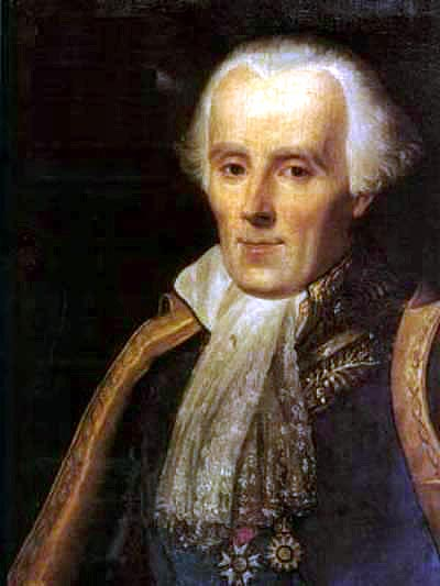
Figure: Pierre-Simon Laplace 1749-1827.

Laplace’s Determism

Figure: Laplace’s determinism book reference.

Famously, Laplace considered the idea of a deterministic Universe, one in which the model is known, or as the below translation refers to it, “an intelligence which could comprehend all the forces by which nature is animated”. He speculates on an “intelligence” that can submit this vast data to analysis and propsoses that such an entity would be able to predict the future.

Given for one instant an intelligence which could comprehend all the forces by which nature is animated and the respective situation of the beings who compose it—an intelligence sufficiently vast to submit these data to analysis—it would embrace in the same formulate the movements of the greatest bodies of the universe and those of the lightest atom; for it, nothing would be uncertain and the future, as the past, would be present in its eyes.

This notion is known as Laplace’s demon or Laplace’s superman.

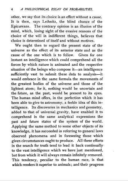
Figure: Laplace’s determinsim in English translation.

Laplace’s Gremlin

Unfortunately, most analyses of his ideas stop at that point, whereas his real point is that such a notion is unreachable. Not so much superman as strawman. Just three pages later in the “Philosophical Essay on Probabilities” (Laplace, 1814), Laplace goes on to observe:

The curve described by a simple molecule of air or vapor is regulated in a manner just as certain as the planetary orbits; the only difference between them is that which comes from our ignorance.

Probability is relative, in part to this ignorance, in part to our knowledge.

Figure: Laplace’s gremlin in the original French.

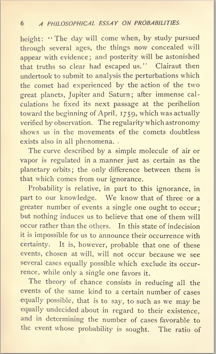
Figure: To Laplace, determinism is a strawman. Ignorance of mechanism and data leads to uncertainty which should be dealt with through probability.

In other words, we can never make use of the idealistic deterministic Universe due to our ignorance about the world, Laplace’s suggestion, and focus in this essay is that we turn to probability to deal with this uncertainty. This is also our inspiration for using probability in machine learning. This is the true message of Laplace’s essay, not determinism, but the gremlin of uncertainty that emerges from our ignorance.

The “forces by which nature is animated” is our model, the “situation of beings that compose it” is our data and the “intelligence sufficiently vast enough to submit these data to analysis” is our compute. The fly in the ointment is our ignorance about these aspects. And probability is the tool we use to incorporate this ignorance leading to uncertainty or doubt in our predictions.

Latent Variables

Laplace’s concept was that the reason that the data doesn’t match up to the model is because of unconsidered factors, and that these might be well represented through probability densities. He tackles the challenge of the unknown factors by adding a variable, \(\epsilon\), that represents the unknown. In modern parlance we would call this a latent variable. But in the context Laplace uses it, the variable is so common that it has other names such as a “slack” variable or the noise in the system.

point 1: \(x= 1\), \(y=3\) \[ 3 = m + c + \epsilon_1 \] point 2: \(x= 3\), \(y=1\) \[ 1 = 3m + c + \epsilon_2 \] point 3: \(x= 2\), \(y=2.5\) \[ 2.5 = 2m + c + \epsilon_3 \]

Laplace’s trick has converted the overdetermined system into an underdetermined system. He has now added three variables, \(\{\epsilon_i\}_{i=1}^3\), which represent the unknown corruptions of the real world. Laplace’s idea is that we should represent that unknown corruption with a probability distribution.

A Probabilistic Process

However, it was left to an admirer of Laplace to develop a practical probability density for that purpose. It was Carl Friedrich Gauss who suggested that the Gaussian density (which at the time was unnamed!) should be used to represent this error.

The result is a noisy function, a function which has a deterministic part, and a stochastic part. This type of function is sometimes known as a probabilistic or stochastic process, to distinguish it from a deterministic process.

Two Important Gaussian Properties

The Gaussian density has many important properties, but for the moment we’ll review two of them.

Sum of Gaussians

If we assume that a variable, \(y_i\), is sampled from a Gaussian density,

\[y_i \sim \mathscr{N}\left(\mu_i,\sigma_i^2\right)\]

Then we can show that the sum of a set of variables, each drawn independently from such a density is also distributed as Gaussian. The mean of the resulting density is the sum of the means, and the variance is the sum of the variances,

\[ \sum_{i=1}^{n} y_i \sim \mathscr{N}\left(\sum_{i=1}^n\mu_i,\sum_{i=1}^n\sigma_i^2\right) \]

Since we are very familiar with the Gaussian density and its properties, it is not immediately apparent how unusual this is. Most random variables, when you add them together, change the family of density they are drawn from. For example, the Gaussian is exceptional in this regard. Indeed, other random variables, if they are independently drawn and summed together tend to a Gaussian density. That is the central limit theorem which is a major justification for the use of a Gaussian density.

Scaling a Gaussian

Less unusual is the scaling property of a Gaussian density. If a variable, \(y\), is sampled from a Gaussian density,

\[y\sim \mathscr{N}\left(\mu,\sigma^2\right)\] and we choose to scale that variable by a deterministic value, \(w\), then the scaled variable is distributed as

\[wy\sim \mathscr{N}\left(w\mu,w^2 \sigma^2\right).\] Unlike the summing properties, where adding two or more random variables independently sampled from a family of densitites typically brings the summed variable outside that family, scaling many densities leaves the distribution of that variable in the same family of densities. Indeed, many densities include a scale parameter (e.g. the Gamma density) which is purely for this purpose. In the Gaussian the standard deviation, \(\sigma\), is the scale parameter. To see why this makes sense, let’s consider, \[z \sim \mathscr{N}\left(0,1\right),\] then if we scale by \(\sigma\) so we have, \(y=\sigma z\), we can write, \[y=\sigma z \sim \mathscr{N}\left(0,\sigma^2\right)\]

Let’s first of all review the properties of the multivariate Gaussian distribution that make linear Gaussian models easier to deal with. We’ll return to the, perhaps surprising, result on the parameters within the nonlinearity, \(\boldsymbol{ \theta}\), shortly.

To work with linear Gaussian models, to find the marginal likelihood all you need to know is the following rules. If \[ \mathbf{ y}= \mathbf{W}\mathbf{ x}+ \boldsymbol{ \epsilon}, \] where \(\mathbf{ y}\), \(\mathbf{ x}\) and \(\boldsymbol{ \epsilon}\) are vectors and we assume that \(\mathbf{ x}\) and \(\boldsymbol{ \epsilon}\) are drawn from multivariate Gaussians, \[ \begin{align} \mathbf{ x}& \sim \mathscr{N}\left(\boldsymbol{ \mu},\mathbf{C}\right)\\ \boldsymbol{ \epsilon}& \sim \mathscr{N}\left(\mathbf{0},\boldsymbol{ \Sigma}\right) \end{align} \] then we know that \(\mathbf{ y}\) is also drawn from a multivariate Gaussian with, \[ \mathbf{ y}\sim \mathscr{N}\left(\mathbf{W}\boldsymbol{ \mu},\mathbf{W}\mathbf{C}\mathbf{W}^\top + \boldsymbol{ \Sigma}\right). \]

With appropriately defined covariance, \(\boldsymbol{ \Sigma}\), this is actually the marginal likelihood for Factor Analysis, or Probabilistic Principal Component Analysis (Tipping and Bishop, 1999), because we integrated out the inputs (or latent variables they would be called in that case).

Laplace’s Idea

Laplace had the idea to augment the observations by noise, that is equivalent to considering a probability density whose mean is given by the prediction function \[p\left(y_i|x_i\right)=\frac{1}{\sqrt{2\pi\sigma^2}}\exp\left(-\frac{\left(y_i-f\left(x_i\right)\right)^{2}}{2\sigma^2}\right).\]

This is known as stochastic process. It is a function that is corrupted by noise. Laplace didn’t suggest the Gaussian density for that purpose, that was an innovation from Carl Friederich Gauss, which is what gives the Gaussian density its name.

Height as a Function of Weight

In the standard Gaussian, parameterized by mean and variance, make the mean a linear function of an input.

This leads to a regression model. \[ \begin{align*} y_i=&f\left(x_i\right)+\epsilon_i,\\ \epsilon_i \sim & \mathscr{N}\left(0,\sigma^2\right). \end{align*} \]

Assume \(y_i\) is height and \(x_i\) is weight.

Olympic Marathon Data

• Gold medal times for Olympic Marathon since 1896.
• Marathons before 1924 didn’t have a standardized distance.
• Present results using pace per km.
• In 1904 Marathon was badly organized leading to very slow times.

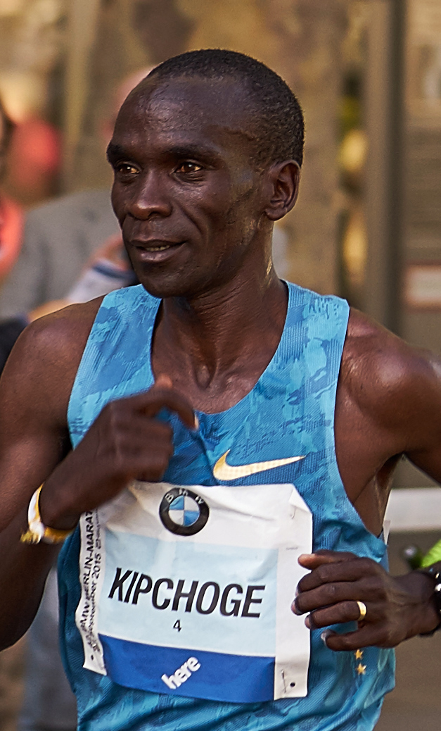
Image from Wikimedia Commons

The Olympic Marathon data is a standard dataset for regression modelling. The data consists of the pace of Olympic Gold Medal Marathon winners for the Olympics from 1896 to present. Let’s load in the data and plot.

cmd = install_command('pods')

%system {cmd}

import numpy as np
import pods

data = pods.datasets.olympic_marathon_men()
x = data['X']
y = data['Y']

offset = y.mean()
scale = np.sqrt(y.var())
yhat = (y - offset)/scale

Figure: Olympic marathon pace times since 1896.

Things to notice about the data include the outlier in 1904, in that year the Olympics was in St Louis, USA. Organizational problems and challenges with dust kicked up by the cars following the race meant that participants got lost, and only very few participants completed. More recent years see more consistently quick marathons.

Running Example: Olympic Marathons

Note that x and y are not pandas data frames for this example, they are just arrays of dimensionality \(n\times 1\), where \(n\) is the number of data.

The aim of this lab is to have you coding linear regression in python. We will do it in two ways, once using iterative updates (coordinate ascent) and then using linear algebra. The linear algebra approach will not only work much better, it is also easy to extend to multiple input linear regression and non-linear regression using basis functions.

Maximum Likelihood: Iterative Solution

Now we will take the maximum likelihood approach we derived in the lecture to fit a line, \(y_i=mx_i + c\), to the data you’ve plotted. We are trying to minimize the error function, \[ E(m, c) = \sum_{i=1}^n(y_i-mx_i-c)^2, \] with respect to \(m\), \(c\) and \(\sigma^2\). We can start with an initial guess for \(m\),

m = -0.4
c = 80

Then we use the maximum likelihood update to find an estimate for the offset, \(c\).

Log Likelihood for Multivariate Regression

Quadratic Loss

Now we’ve identified the empirical risk with the loss, we’ll use \(E(\mathbf{ w})\) to represent our objective function. \[ E(\mathbf{ w}) = \sum_{i=1}^n\left(y_i - f(\mathbf{ x}_i, \mathbf{ w})\right)^2 \] gives us our objective.

In the case of the linear prediction function, we can substitute \(f(\mathbf{ x}_i, \mathbf{ w}) = \mathbf{ w}^\top \mathbf{ x}_i\). \[ E(\mathbf{ w}) = \sum_{i=1}^n\left(y_i - \mathbf{ w}^\top \mathbf{ x}_i\right)^2 \] To compute the gradient of the objective, we first expand the brackets.

Bracket Expansion

\[ \begin{align*} E(\mathbf{ w},\sigma^2) = & \frac{n}{2}\log \sigma^2 + \frac{1}{2\sigma^2}\sum _{i=1}^{n}y_i^{2}-\frac{1}{\sigma^2}\sum _{i=1}^{n}y_i\mathbf{ w}^{\top}\mathbf{ x}_i\\&+\frac{1}{2\sigma^2}\sum _{i=1}^{n}\mathbf{ w}^{\top}\mathbf{ x}_i\mathbf{ x}_i^{\top}\mathbf{ w} +\text{const}.\\ = & \frac{n}{2}\log \sigma^2 + \frac{1}{2\sigma^2}\sum _{i=1}^{n}y_i^{2}-\frac{1}{\sigma^2} \mathbf{ w}^\top\sum_{i=1}^{n}\mathbf{ x}_iy_i\\&+\frac{1}{2\sigma^2} \mathbf{ w}^{\top}\left[\sum _{i=1}^{n}\mathbf{ x}_i\mathbf{ x}_i^{\top}\right]\mathbf{ w}+\text{const}. \end{align*} \]

Solution with Linear Algebra

In this section we’re going compute the minimum of the quadratic loss with respect to the parameters. When we do this, we’ll also review linear algebra. We will represent all our errors and functions in the form of matrices and vectors.

Linear algebra is just a shorthand for performing lots of multiplications and additions simultaneously. What does it have to do with our system then? Well, the first thing to note is that the classic linear function we fit for a one-dimensional regression has the form: \[ f(x) = mx + c \] the classical form for a straight line. From a linear algebraic perspective, we are looking for multiplications and additions. We are also looking to separate our parameters from our data. The data is the givens. In French the word is données literally translated means givens that’s great, because we don’t need to change the data, what we need to change are the parameters (or variables) of the model. In this function the data comes in through \(x\), and the parameters are \(m\) and \(c\).

What we’d like to create is a vector of parameters and a vector of data. Then we could represent the system with vectors that represent the data, and vectors that represent the parameters.

We look to turn the multiplications and additions into a linear algebraic form, we have one multiplication (\(m\times c\)) and one addition (\(mx + c\)). But we can turn this into an inner product by writing it in the following way, \[ f(x) = m \times x + c \times 1, \] in other words, we’ve extracted the unit value from the offset, \(c\). We can think of this unit value like an extra item of data, because it is always given to us, and it is always set to 1 (unlike regular data, which is likely to vary!). We can therefore write each input data location, \(\mathbf{ x}\), as a vector \[ \mathbf{ x}= \begin{bmatrix} 1\\ x\end{bmatrix}. \]

Now we choose to also turn our parameters into a vector. The parameter vector will be defined to contain \[ \mathbf{ w}= \begin{bmatrix} c \\ m\end{bmatrix} \] because if we now take the inner product between these two vectors we recover \[ \mathbf{ x}\cdot\mathbf{ w}= 1 \times c + x \times m = mx + c \] In numpy we can define this vector as follows

import numpy as np

# define the vector w
w = np.zeros(shape=(2, 1))
w[0] = m
w[1] = c

This gives us the equivalence between original operation and an operation in vector space. Whilst the notation here isn’t a lot shorter, the beauty is that we will be able to add as many features as we like and keep the same representation. In general, we are now moving to a system where each of our predictions is given by an inner product. When we want to represent a linear product in linear algebra, we tend to do it with the transpose operation, so since we have \(\mathbf{a}\cdot\mathbf{b} = \mathbf{a}^\top\mathbf{b}\) we can write \[ f(\mathbf{ x}_i) = \mathbf{ x}_i^\top\mathbf{ w}. \] Where we’ve assumed that each data point, \(\mathbf{ x}_i\), is now written by appending a 1 onto the original vector \[ \mathbf{ x}_i = \begin{bmatrix} 1 \\ x_i \end{bmatrix} \]

Design Matrix

We can do this for the entire data set to form a design matrix \(\boldsymbol{ \Phi}\), \[ \boldsymbol{ \Phi} = \begin{bmatrix} \mathbf{ x}_1^\top \\\ \mathbf{ x}_2^\top \\\ \vdots \\\ \mathbf{ x}_n^\top \end{bmatrix} = \begin{bmatrix} 1 & x_1 \\\ 1 & x_2 \\\ \vdots & \vdots \\\ 1 & x_n \end{bmatrix}, \] which in numpy can be done with the following commands:

import numpy as np

Phi = np.hstack((np.ones_like(x), x))
print(Phi)

Writing the Objective with Linear Algebra

When we think of the objective function, we can think of it as the errors where the error is defined in a similar way to what it was in Legendre’s day \(y_i - f(\mathbf{ x}_i)\), in statistics these errors are also sometimes called residuals. So, we can think as the objective and the prediction function as two separate parts, first we have, \[ E(\mathbf{ w}) = \sum_{i=1}^n(y_i - f(\mathbf{ x}_i; \mathbf{ w}))^2, \] where we’ve made the function \(f(\cdot)\)’s dependence on the parameters \(\mathbf{ w}\) explicit in this equation. Then we have the definition of the function itself, \[ f(\mathbf{ x}_i; \mathbf{ w}) = \mathbf{ x}_i^\top \mathbf{ w}. \] Let’s look again at these two equations and see if we can identify any inner products. The first equation is a sum of squares, which is promising. Any sum of squares can be represented by an inner product, \[ a = \sum_{i=1}^{k} b^2_i = \mathbf{b}^\top\mathbf{b}. \] If we wish to represent \(E(\mathbf{ w})\) in this way, all we need to do is convert the sum operator to an inner product. We can get a vector from that sum operator by placing both \(y_i\) and \(f(\mathbf{ x}_i; \mathbf{ w})\) into vectors, which we do by defining \[ \mathbf{ y}= \begin{bmatrix}y_1\\ y_2\\ \vdots \\ y_n\end{bmatrix} \] and defining \[ \mathbf{ f}(\mathbf{ x}_1; \mathbf{ w}) = \begin{bmatrix}f(\mathbf{ x}_1; \mathbf{ w})\\ f(\mathbf{ x}_2; \mathbf{ w})\\ \vdots \\ f(\mathbf{ x}_n; \mathbf{ w})\end{bmatrix}. \] The second of these is a vector-valued function. This term may appear intimidating, but the idea is straightforward. A vector valued function is simply a vector whose elements are themselves defined as functions, i.e., it is a vector of functions, rather than a vector of scalars. The idea is so straightforward, that we are going to ignore it for the moment, and barely use it in the derivation. But it will reappear later when we introduce basis functions. So, we will for the moment ignore the dependence of \(\mathbf{ f}\) on \(\mathbf{ w}\) and \(\boldsymbol{ \Phi}\) and simply summarise it by a vector of numbers \[ \mathbf{ f}= \begin{bmatrix}f_1\\f_2\\ \vdots \\ f_n\end{bmatrix}. \] This allows us to write our objective in the folowing, linear algebraic form, \[ E(\mathbf{ w}) = (\mathbf{ y}- \mathbf{ f})^\top(\mathbf{ y}- \mathbf{ f}) \] from the rules of inner products. But what of our matrix \(\boldsymbol{ \Phi}\) of input data? At this point, we need to dust off matrix-vector multiplication. Matrix multiplication is simply a convenient way of performing many inner products together, and it’s exactly what we need to summarize the operation \[ f_i = \mathbf{ x}_i^\top\mathbf{ w}. \] This operation tells us that each element of the vector \(\mathbf{ f}\) (our vector valued function) is given by an inner product between \(\mathbf{ x}_i\) and \(\mathbf{ w}\). In other words, it is a series of inner products. Let’s look at the definition of matrix multiplication, it takes the form \[ \mathbf{c} = \mathbf{B}\mathbf{a}, \] where \(\mathbf{c}\) might be a \(k\) dimensional vector (which we can interpret as a \(k\times 1\) dimensional matrix), and \(\mathbf{B}\) is a \(k\times k\) dimensional matrix and \(\mathbf{a}\) is a \(k\) dimensional vector (\(k\times 1\) dimensional matrix).

The result of this multiplication is of the form \[ \begin{bmatrix}c_1\\c_2 \\ \vdots \\ a_k\end{bmatrix} = \begin{bmatrix} b_{1,1} & b_{1, 2} & \dots & b_{1, k} \\ b_{2, 1} & b_{2, 2} & \dots & b_{2, k} \\ \vdots & \vdots & \ddots & \vdots \\ b_{k, 1} & b_{k, 2} & \dots & b_{k, k} \end{bmatrix} \begin{bmatrix}a_1\\a_2 \\ \vdots\\ c_k\end{bmatrix} = \begin{bmatrix} b_{1, 1}a_1 + b_{1, 2}a_2 + \dots + b_{1, k}a_k\\ b_{2, 1}a_1 + b_{2, 2}a_2 + \dots + b_{2, k}a_k \\ \vdots\\ b_{k, 1}a_1 + b_{k, 2}a_2 + \dots + b_{k, k}a_k\end{bmatrix}. \] We see that each element of the result, \(\mathbf{a}\) is simply the inner product between each row of \(\mathbf{B}\) and the vector \(\mathbf{c}\). Because we have defined each element of \(\mathbf{ f}\) to be given by the inner product between each row of the design matrix and the vector \(\mathbf{ w}\) we now can write the full operation in one matrix multiplication,

\[ \mathbf{ f}= \boldsymbol{ \Phi}\mathbf{ w}. \]

import numpy as np

f = Phi@w # The @ sign performs matrix multiplication

Combining this result with our objective function, \[ E(\mathbf{ w}) = (\mathbf{ y}- \mathbf{ f})^\top(\mathbf{ y}- \mathbf{ f}) \] we find we have defined the model with two equations. One equation tells us the form of our predictive function and how it depends on its parameters, the other tells us the form of our objective function.

resid = (y-f)
E = np.dot(resid.T, resid) # matrix multiplication on a single vector is equivalent to a dot product.
print("Error function is:", E)

Objective Optimization

Our model has now been defined with two equations: the prediction function and the objective function. Now we will use multivariate calculus to define an algorithm to fit the model. The separation between model and algorithm is important and is often overlooked. Our model contains a function that shows how it will be used for prediction, and a function that describes the objective function we need to optimize to obtain a good set of parameters.

The model linear regression model we have described is still the same as the one we fitted above with a coordinate ascent algorithm. We have only played with the notation to obtain the same model in a matrix and vector notation. However, we will now fit this model with a different algorithm, one that is much faster. It is such a widely used algorithm that from the end user’s perspective it doesn’t even look like an algorithm, it just appears to be a single operation (or function). However, underneath the computer calls an algorithm to find the solution. Further, the algorithm we obtain is very widely used, and because of this it turns out to be highly optimized.

Once again, we are going to try and find the stationary points of our objective by finding the stationary points. However, the stationary points of a multivariate function, are a little bit more complex to find. As before we need to find the point at which the gradient is zero, but now we need to use multivariate calculus to find it. This involves learning a few additional rules of differentiation (that allow you to do the derivatives of a function with respect to vector), but in the end it makes things quite a bit easier. We define vectorial derivatives as follows, \[ \frac{\text{d}E(\mathbf{ w})}{\text{d}\mathbf{ w}} = \begin{bmatrix}\frac{\text{d}E(\mathbf{ w})}{\text{d}w_1}\\\frac{\text{d}E(\mathbf{ w})}{\text{d}w_2}\end{bmatrix}. \] where \(\frac{\text{d}E(\mathbf{ w})}{\text{d}w_1}\) is the partial derivative of the error function with respect to \(w_1\).

Differentiation through multiplications and additions is relatively straightforward, and since linear algebra is just multiplication and addition, then its rules of differentiation are quite straightforward too, but slightly more complex than regular derivatives.

Multivariate Derivatives

We will need two rules of multivariate or matrix differentiation. The first is differentiation of an inner product. By remembering that the inner product is made up of multiplication and addition, we can hope that its derivative is quite straightforward, and so it proves to be. We can start by thinking about the definition of the inner product, \[ \mathbf{a}^\top\mathbf{z} = \sum_{i} a_i z_i, \] which if we were to take the derivative with respect to \(z_k\) would simply return the gradient of the one term in the sum for which the derivative was non-zero, that of \(a_k\), so we know that \[ \frac{\text{d}}{\text{d}z_k} \mathbf{a}^\top \mathbf{z} = a_k \] and by our definition for multivariate derivatives, we can simply stack all the partial derivatives of this form in a vector to obtain the result that \[ \frac{\text{d}}{\text{d}\mathbf{z}} \mathbf{a}^\top \mathbf{z} = \mathbf{a}. \] The second rule that’s required is differentiation of a ‘matrix quadratic’. A scalar quadratic in \(z\) with coefficient \(c\) has the form \(cz^2\). If \(\mathbf{z}\) is a \(k\times 1\) vector and \(\mathbf{C}\) is a \(k \times k\) matrix of coefficients then the matrix quadratic form is written as \(\mathbf{z}^\top \mathbf{C}\mathbf{z}\), which is itself a scalar quantity, but it is a function of a vector.

Matching Dimensions in Matrix Multiplications

There’s a trick for telling a multiplication leads to a scalar result. When you are doing mathematics with matrices, it’s always worth pausing to perform a quick sanity check on the dimensions. Matrix multplication only works when the dimensions match. To be precise, the ‘inner’ dimension of the matrix must match. What is the inner dimension? If we multiply two matrices \(\mathbf{A}\) and \(\mathbf{B}\), the first of which has \(k\) rows and \(\ell\) columns and the second of which has \(p\) rows and \(q\) columns, then we can check whether the multiplication works by writing the dimensionalities next to each other, \[ \mathbf{A} \mathbf{B} \rightarrow (k \times \underbrace{\ell)(p}_\text{inner dimensions} \times q) \rightarrow (k\times q). \] The inner dimensions are the two inside dimensions, \(\ell\) and \(p\). The multiplication will only work if \(\ell=p\). The result of the multiplication will then be a \(k\times q\) matrix: this dimensionality comes from the ‘outer dimensions’. Note that matrix multiplication is not commutative. And if you change the order of the multiplication, \[ \mathbf{B} \mathbf{A} \rightarrow (\ell \times \underbrace{k)(q}_\text{inner dimensions} \times p) \rightarrow (\ell \times p). \] Firstly, it may no longer even work, because now the condition is that \(k=q\), and secondly the result could be of a different dimensionality. An exception is if the matrices are square matrices (e.g., same number of rows as columns) and they are both symmetric. A symmetric matrix is one for which \(\mathbf{A}=\mathbf{A}^\top\), or equivalently, \(a_{i,j} = a_{j,i}\) for all \(i\) and \(j\).

For applying and developing machine learning algorithms you should get familiar with working with matrices and vectors. You should have come across them before, but you may not have used them as extensively as we are doing now. It’s worth getting used to using this trick to check your work and ensure you know what the dimension of an output matrix should be. For our matrix quadratic form, it turns out that we can see it as a special type of inner product. \[ \mathbf{z}^\top\mathbf{C}\mathbf{z} \rightarrow (1\times \underbrace{k) (k}_\text{inner dimensions}\times k) (k\times 1) \rightarrow \mathbf{b}^\top\mathbf{z} \] where \(\mathbf{b} = \mathbf{C}\mathbf{z}\) so therefore the result is a scalar, \[ \mathbf{b}^\top\mathbf{z} \rightarrow (1\times \underbrace{k) (k}_\text{inner dimensions}\times 1) \rightarrow (1\times 1) \] where a \((1\times 1)\) matrix is recognised as a scalar.

This implies that we should be able to differentiate this form, and indeed the rule for its differentiation is slightly more complex than the inner product, but still quite simple, \[ \frac{\text{d}}{\text{d}\mathbf{z}} \mathbf{z}^\top\mathbf{C}\mathbf{z}= \mathbf{C}\mathbf{z} + \mathbf{C}^\top \mathbf{z}. \] Note that in the special case where \(\mathbf{C}\) is symmetric then we have \(\mathbf{C} = \mathbf{C}^\top\) and the derivative simplifies to \[ \frac{\text{d}}{\text{d}\mathbf{z}} \mathbf{z}^\top\mathbf{C}\mathbf{z}= 2\mathbf{C}\mathbf{z}. \]

Differentiate the Objective

First, we need to compute the full objective by substituting our prediction function into the objective function to obtain the objective in terms of \(\mathbf{ w}\). Doing this we obtain \[ E(\mathbf{ w})= (\mathbf{ y}- \boldsymbol{ \Phi}\mathbf{ w})^\top (\mathbf{ y}- \boldsymbol{ \Phi}\mathbf{ w}). \] We now need to differentiate this quadratic form to find the minimum. We differentiate with respect to the vector \(\mathbf{ w}\). But before we do that, we’ll expand the brackets in the quadratic form to obtain a series of scalar terms. The rules for bracket expansion across the vectors are similar to those for the scalar system giving, \[ (\mathbf{a} - \mathbf{b})^\top (\mathbf{c} - \mathbf{d}) = \mathbf{a}^\top \mathbf{c} - \mathbf{a}^\top \mathbf{d} - \mathbf{b}^\top \mathbf{c} + \mathbf{b}^\top \mathbf{d} \] which substituting for \(\mathbf{a} = \mathbf{c} = \mathbf{ y}\) and \(\mathbf{b}=\mathbf{d} = \boldsymbol{ \Phi}\mathbf{ w}\) gives \[ E(\mathbf{ w})= \mathbf{ y}^\top\mathbf{ y}- 2\mathbf{ y}^\top\boldsymbol{ \Phi}\mathbf{ w}+ \mathbf{ w}^\top\boldsymbol{ \Phi}^\top\boldsymbol{ \Phi}\mathbf{ w} \] where we used the fact that \(\mathbf{ y}^\top\boldsymbol{ \Phi}\mathbf{ w}=\mathbf{ w}^\top\boldsymbol{ \Phi}^\top\mathbf{ y}\).

Now we can use our rules of differentiation to compute the derivative of this form, which is, \[ \frac{\text{d}}{\text{d}\mathbf{ w}}E(\mathbf{ w})=- 2\boldsymbol{ \Phi}^\top \mathbf{ y}+ 2\boldsymbol{ \Phi}^\top\boldsymbol{ \Phi}\mathbf{ w}, \] where we have exploited the fact that \(\boldsymbol{ \Phi}^\top\boldsymbol{ \Phi}\) is symmetric to obtain this result.

Exercise 1

Use the equivalence between our vector and our matrix formulations of linear regression, alongside our definition of vector derivates, to match the gradients we’ve computed directly for \(\frac{\text{d}E(c, m)}{\text{d}c}\) and \(\frac{\text{d}E(c, m)}{\text{d}m}\) to those for \(\frac{\text{d}E(\mathbf{ w})}{\text{d}\mathbf{ w}}\).

Update Equation for Global Optimum

We need to find the minimum of our objective function. Using our objective function, we can minimize for our parameter vector \(\mathbf{ w}\). Firstly, we seek stationary points by find parameter vectors that solve for when the gradients are zero, \[ \mathbf{0}=- 2\boldsymbol{ \Phi}^\top \mathbf{ y}+ 2\boldsymbol{ \Phi}^\top\boldsymbol{ \Phi}\mathbf{ w}, \] where \(\mathbf{0}\) is a vector of zeros. Rearranging this equation, we find the solution to be \[ \boldsymbol{ \Phi}^\top \boldsymbol{ \Phi}\mathbf{ w}= \boldsymbol{ \Phi}^\top \mathbf{ y} \] which is a matrix equation of the familiar form \(\mathbf{A}\mathbf{x} = \mathbf{b}\).

Solving the Multivariate System

The solution for \(\mathbf{ w}\) can be written mathematically in terms of a matrix inverse of \(\boldsymbol{ \Phi}^\top\boldsymbol{ \Phi}\), but computation of a matrix inverse requires an algorithm to resolve it. You’ll know this if you had to invert, by hand, a \(3\times 3\) matrix in high school. From a numerical stability perspective, it is also best not to compute the matrix inverse directly, but rather to ask the computer to solve the system of linear equations given by \[ \boldsymbol{ \Phi}^\top\boldsymbol{ \Phi}\mathbf{ w}= \boldsymbol{ \Phi}^\top\mathbf{ y} \] for \(\mathbf{ w}\).

Multivariate Linear Regression

A major advantage of the new system is that we can build a linear regression on a multivariate system. The matrix calculus didn’t specify what the length of the vector \(\mathbf{ x}\) should be, or equivalently the size of the design matrix.

Movie Violence Data

This is a data set created by Simon Garnier and Rany Olson for exploring the differences between R and Python for data science. The data contains information about different movies augmented by estimates about how many on-screen deaths are contained in the movie. The data is craped from http://www.moviebodycounts.com. The data contains the following featuers for each movie: Year, Body_Count, MPAA_Rating, Genre, Director, Actors, Length_Minutes, IMDB_Rating.

import pods

data = pods.datasets.movie_body_count()
movies = data['Y']

The data is provided to us in the form of a pandas data frame, we can see the features we’re provided with by inspecting the columns of the data frame.

print(', '.join(movies.columns))

Once it is loaded in the data can be summarized using the describe method in pandas.

Multivariate Regression on Movie Violence Data

Now we will build a design matrix based on the numeric features: year, Body_Count, Length_Minutes in an effort to predict the rating. We build the design matrix as follows:

Bias as an additional feature.

select_features = ['Year', 'Body_Count', 'Length_Minutes']
Phi = movies[select_features].copy()
Phi['Eins'] = 1 # add a column for the offset
y = movies[['IMDB_Rating']]

Now let’s perform a linear regression. But this time, we will create a pandas data frame for the result so we can store it in a form that we can visualise easily.

import numpy as np
import pandas as pd

solution = np.linalg.solve(Phi.T@Phi, Phi.T@y) # solve linear regression here
# Place the solution in the data frame
w = pd.DataFrame(data=solution, 
                 index = Phi.columns,  # columns of Phi become rows of w
                 columns=['regression_coefficient']) # the column of Phi is the value of regression coefficient

We can check the residuals to see how good our estimates are. First we create a pandas data frame containing the predictions and use it to compute the residuals.

ypred = pd.DataFrame(data=(Phi@w).values, columns=['IMDB_Rating'])
resid = y-ypred

Figure: Residual values for the ratings from the prediction of the movie rating given the data from the film.

Which shows our model hasn’t yet done a great job of representation, because the spread of values is large. We can check what the rating is dominated by in terms of regression coefficients.

w

Although we have to be a little careful about interpretation because our input values live on different scales, however it looks like we are dominated by the bias, with a small negative effect for later films (but bear in mind the years are large, so this effect is probably larger than it looks) and a positive effect for length. So it looks like long earlier films generally do better, but the residuals are so high that we probably haven’t modelled the system very well.

Underdetermined System

What about the situation where you have more parameters than data in your simultaneous equation? This is known as an underdetermined system. In fact, this set up is in some sense easier to solve, because we don’t need to think about introducing a slack variable (although it might make a lot of sense from a modelling perspective to do so).

The way Laplace proposed resolving an overdetermined system, was to introduce slack variables, \(\epsilon_i\), which needed to be estimated for each point. The slack variable represented the difference between our actual prediction and the true observation. This is known as the residual. By introducing the slack variable, we now have an additional \(n\) variables to estimate, one for each data point, \(\{\epsilon_i\}\). This turns the overdetermined system into an underdetermined system. Introduction of \(n\) variables, plus the original \(m\) and \(c\) gives us \(n+2\) parameters to be estimated from \(n\) observations, which makes the system underdetermined. However, we then made a probabilistic assumption about the slack variables, we assumed that the slack variables were distributed according to a probability density. And for the moment we have been assuming that density was the Gaussian, \[\epsilon_i \sim \mathscr{N}\left(0,\sigma^2\right),\] with zero mean and variance \(\sigma^2\).

The follow up question is whether we can do the same thing with the parameters. If we have two parameters and only one unknown, can we place a probability distribution over the parameters as we did with the slack variables? The answer is yes.

Underdetermined System

Figure: An underdetermined system can be fit by considering uncertainty. Multiple solutions are consistent with one specified point.

Two Dimensional Gaussian

Consider the distribution of height (in meters) of an adult male human population. We will approximate the marginal density of heights as a Gaussian density with mean given by \(1.7\text{m}\) and a standard deviation of \(0.15\text{m}\), implying a variance of \(\sigma^2=0.0225\), \[ p(h) \sim \mathscr{N}\left(1.7,0.0225\right). \] Similarly, we assume that weights of the population are distributed a Gaussian density with a mean of \(75 \text{kg}\) and a standard deviation of \(6 kg\) (implying a variance of 36), \[ p(w) \sim \mathscr{N}\left(75,36\right). \]

Figure: Gaussian distributions for height and weight.

Independence Assumption

First of all, we make an independence assumption, we assume that height and weight are independent. The definition of probabilistic independence is that the joint density, \(p(w, h)\), factorizes into its marginal densities, \[ p(w, h) = p(w)p(h). \] Given this assumption we can sample from the joint distribution by independently sampling weights and heights.

displaycode{nu.display_plots(‘independent_height_weight{fig:0>3}.svg’, directory=‘./ml’, fig=IntSlider(0, 0, 7, 1))}

Figure: Samples from independent Gaussian variables that might represent heights and weights.

In reality height and weight are not independent. Taller people tend on average to be heavier, and heavier people are likely to be taller. This is reflected by the body mass index. A ratio suggested by one of the fathers of statistics, Adolphe Quetelet. Quetelet was interested in the notion of the average man and collected various statistics about people. He defined the BMI to be, \[ \text{BMI} = \frac{w}{h^2} \]To deal with this dependence we now introduce the notion of correlation to the multivariate Gaussian density.

Sampling Two Dimensional Variables

Figure: Samples from correlated Gaussian variables that might represent heights and weights.

Independent Gaussians

\[ p(w, h) = p(w)p(h) \]

\[ p(w, h) = \frac{1}{\sqrt{2\pi \sigma_1^2}\sqrt{2\pi\sigma_2^2}} \exp\left(-\frac{1}{2}\left(\frac{(w-\mu_1)^2}{\sigma_1^2} + \frac{(h-\mu_2)^2}{\sigma_2^2}\right)\right) \]

\[ p(w, h) = \frac{1}{\sqrt{2\pi\sigma_1^22\pi\sigma_2^2}} \exp\left(-\frac{1}{2}\left(\begin{bmatrix}w \\ h\end{bmatrix} - \begin{bmatrix}\mu_1 \\ \mu_2\end{bmatrix}\right)^\top\begin{bmatrix}\sigma_1^2& 0\\0&\sigma_2^2\end{bmatrix}^{-1}\left(\begin{bmatrix}w \\ h\end{bmatrix} - \begin{bmatrix}\mu_1 \\ \mu_2\end{bmatrix}\right)\right) \]

\[ p(\mathbf{ y}) = \frac{1}{\det{2\pi \mathbf{D}}^{\frac{1}{2}}} \exp\left(-\frac{1}{2}(\mathbf{ y}- \boldsymbol{ \mu})^\top\mathbf{D}^{-1}(\mathbf{ y}- \boldsymbol{ \mu})\right) \]

Correlated Gaussian

Form correlated from original by rotating the data space using matrix \(\mathbf{R}\).

\[ p(\mathbf{ y}) = \frac{1}{\det{2\pi\mathbf{D}}^{\frac{1}{2}}} \exp\left(-\frac{1}{2}(\mathbf{ y}- \boldsymbol{ \mu})^\top\mathbf{D}^{-1}(\mathbf{ y}- \boldsymbol{ \mu})\right) \]

\[ p(\mathbf{ y}) = \frac{1}{\det{2\pi\mathbf{D}}^{\frac{1}{2}}} \exp\left(-\frac{1}{2}(\mathbf{R}^\top\mathbf{ y}- \mathbf{R}^\top\boldsymbol{ \mu})^\top\mathbf{D}^{-1}(\mathbf{R}^\top\mathbf{ y}- \mathbf{R}^\top\boldsymbol{ \mu})\right) \]

\[ p(\mathbf{ y}) = \frac{1}{\det{2\pi\mathbf{D}}^{\frac{1}{2}}} \exp\left(-\frac{1}{2}(\mathbf{ y}- \boldsymbol{ \mu})^\top\mathbf{R}\mathbf{D}^{-1}\mathbf{R}^\top(\mathbf{ y}- \boldsymbol{ \mu})\right) \] this gives an inverse covariance matrix: \[ \mathbf{C}^{-1} = \mathbf{R}\mathbf{D}^{-1} \mathbf{R}^\top \]

\[ p(\mathbf{ y}) = \frac{1}{\det{2\pi\mathbf{C}}^{\frac{1}{2}}} \exp\left(-\frac{1}{2}(\mathbf{ y}- \boldsymbol{ \mu})^\top\mathbf{C}^{-1} (\mathbf{ y}- \boldsymbol{ \mu})\right) \] \[ \mathbf{C}= \mathbf{R}\mathbf{D} \mathbf{R}^\top \]

Basis Functions

Here’s the idea, instead of working directly on the original input space, \(\mathbf{ x}\), we build models in a new space, \(\boldsymbol{ \phi}(\mathbf{ x})\) where \(\boldsymbol{ \phi}(\cdot)\) is a vector-valued function that is defined on the space \(\mathbf{ x}\).

Quadratic Basis

Remember, that a vector-valued function is just a vector that contains functions instead of values. Here’s an example for a one dimensional input space, \(x\), being projected to a quadratic basis. First we consider each basis function in turn, we can think of the elements of our vector as being indexed so that we have \[ \begin{align*} \phi_1(x) & = 1, \\ \phi_2(x) & = x, \\ \phi_3(x) & = x^2. \end{align*} \] Now we can consider them together by placing them in a vector, \[ \boldsymbol{ \phi}(x) = \begin{bmatrix} 1\\ x \\ x^2\end{bmatrix}. \] For the vector-valued function, we have simply collected the different functions together in the same vector making them notationally easier to deal with in our mathematics.

When we consider the vector-valued function for each data point, then we place all the data into a matrix. The result is a matrix valued function, \[ \boldsymbol{ \Phi}(\mathbf{ x}) = \begin{bmatrix} 1 & x_1 & x_1^2 \\ 1 & x_2 & x_2^2\\ \vdots & \vdots & \vdots \\ 1 & x_n & x_n^2 \end{bmatrix} \] where we are still in the one dimensional input setting so \(\mathbf{ x}\) here represents a vector of our inputs with \(n\) elements.

Let’s try constructing such a matrix for a set of inputs. First of all, we create a function that returns the matrix valued function.

import numpy as np

def quadratic(x, **kwargs):
    """Take in a vector of input values and return the design matrix associated 
    with the basis functions."""
    return np.hstack([np.ones((x.shape[0], 1)), x, x**2])

Functions Derived from Quadratic Basis

\[ f(x) = {\color{red}{w_0}} + {\color{magenta}{w_1 x}} + {\color{blue}{w_2 x^2}} \]

Figure: The set of functions which are combined to form a quadratic basis.

This function takes in an \(n\times 1\) dimensional vector and returns an \(n\times 3\) dimensional design matrix containing the basis functions. We can plot those basis functions against there input as follows.

The actual function we observe is then made up of a sum of these functions. This is the reason for the name basis. The term basis means ‘the underlying support or foundation for an idea, argument, or process’, and in this context they form the underlying support for our prediction function. Our prediction function can only be composed of a weighted linear sum of our basis functions.

Quadratic Functions

Figure: Functions constructed by weighted sum of the components of a quadratic basis.

Rectified Linear Units

The rectified linear unit is a basis function that emerged out of the deep learning community. Rectified linear units are popular in the current generation of multilayer perceptron models, or deep networks. These basis functions start flat, and then become linear functions at a certain threshold. \[ \phi_j(x) = xH(x+ v_j) \]

import numpy as np

from mlai import relu

Figure: The set of functions which are combined to form a rectified linear unit basis.

Functions Derived from Relu Basis

\[ f(x) = \color{red}{w_0} + \color{magenta}{w_1 xH(x+1.0) } + \color{blue}{w_2 xH(x+0.33) } + \color{green}{w_3 xH(x-0.33)} + \color{cyan}{w_4 xH(x-1.0)} \]

Figure: A rectified linear unit basis is made up of different rectified linear unit functions centered at different points.

Gaussian Processes

Models where we model the entire joint distribution of our training data, \(p(\mathbf{ y}, \mathbf{X})\) are sometimes described as generative models. Because we can use sampling to generate data sets that represent all our assumptions. However, as we discussed in the sessions on and , this can be a bad idea, because if our assumptions are wrong then we can make poor predictions. We can try to make more complex assumptions about data to alleviate the problem, but then this typically leads to challenges for tractable application of the sum and rules of probability that are needed to compute the relevant marginal and conditional densities. If we know the form of the question we wish to answer then we typically try and represent that directly, through \(p(\mathbf{ y}|\mathbf{X})\). In practice, we also have been making assumptions of conditional independence given the model parameters, \[ p(\mathbf{ y}|\mathbf{X}, \mathbf{ w}) = \prod_{i=1}^{n} p(y_i | \mathbf{ x}_i, \mathbf{ w}) \] Gaussian processes are not normally considered to be generative models, but we will be much more interested in the principles of conditioning in Gaussian processes because we will use conditioning to make predictions between our test and training data. We will avoid the data conditional indpendence assumption in favour of a richer assumption about the data, in a Gaussian process we assume data is jointly Gaussian with a particular mean and covariance, \[ \mathbf{ y}|\mathbf{X}\sim \mathscr{N}\left(\mathbf{m}(\mathbf{X}),\mathbf{K}(\mathbf{X})\right), \] where the conditioning is on the inputs \(\mathbf{X}\) which are used for computing the mean and covariance. For this reason they are known as mean and covariance functions.

Linear Model Overview

However, we are focussing on what happens in models which are non-linear in the inputs, whereas the above would be linear in the inputs. To consider these, we introduce a matrix, called the design matrix. We set each activation function computed at each data point to be \[ \phi_{i,j} = \phi(\mathbf{ w}^{(1)}_{j}, \mathbf{ x}_{i}) \] and define the matrix of activations (known as the design matrix in statistics) to be, \[ \boldsymbol{ \Phi}= \begin{bmatrix} \phi_{1, 1} & \phi_{1, 2} & \dots & \phi_{1, h} \\ \phi_{1, 2} & \phi_{1, 2} & \dots & \phi_{1, n} \\ \vdots & \vdots & \ddots & \vdots \\ \phi_{n, 1} & \phi_{n, 2} & \dots & \phi_{n, h} \end{bmatrix}. \] By convention this matrix always has \(n\) rows and \(h\) columns, now if we define the vector of all noise corruptions, \(\boldsymbol{ \epsilon}= \left[\epsilon_1, \dots \epsilon_n\right]^\top\).

If we define the prior distribution over the vector \(\mathbf{ w}\) to be Gaussian, \[ \mathbf{ w}\sim \mathscr{N}\left(\mathbf{0},\alpha\mathbf{I}\right), \] then we can use rules of multivariate Gaussians to see that, \[ \mathbf{ y}\sim \mathscr{N}\left(\mathbf{0},\alpha \boldsymbol{ \Phi}\boldsymbol{ \Phi}^\top + \sigma^2 \mathbf{I}\right). \]

In other words, our training data is distributed as a multivariate Gaussian, with zero mean and a covariance given by \[ \mathbf{K}= \alpha \boldsymbol{ \Phi}\boldsymbol{ \Phi}^\top + \sigma^2 \mathbf{I}. \]

This is an \(n\times n\) size matrix. Its elements are in the form of a function. The maths shows that any element, index by \(i\) and \(j\), is a function only of inputs associated with data points \(i\) and \(j\), \(\mathbf{ y}_i\), \(\mathbf{ y}_j\). \(k_{i,j} = k\left(\mathbf{ x}_i, \mathbf{ x}_j\right)\)

If we look at the portion of this function associated only with \(f(\cdot)\), i.e. we remove the noise, then we can write down the covariance associated with our neural network, \[ k_f\left(\mathbf{ x}_i, \mathbf{ x}_j\right) = \alpha \boldsymbol{ \phi}\left(\mathbf{W}_1, \mathbf{ x}_i\right)^\top \boldsymbol{ \phi}\left(\mathbf{W}_1, \mathbf{ x}_j\right) \] so the elements of the covariance or kernel matrix are formed by inner products of the rows of the design matrix.

Gaussian Process

This is the essence of a Gaussian process. Instead of making assumptions about our density over each data point, \(y_i\) as i.i.d. we make a joint Gaussian assumption over our data. The covariance matrix is now a function of both the parameters of the activation function, \(\mathbf{V}\), and the input variables, \(\mathbf{X}\). This comes about through integrating out the parameters of the model, \(\mathbf{ w}\).

Basis Functions

We can basically put anything inside the basis functions, and many people do. These can be deep kernels (Cho and Saul, 2009) or we can learn the parameters of a convolutional neural network inside there.

Viewing a neural network in this way is also what allows us to beform sensible batch normalizations (Ioffe and Szegedy, 2015).

Radial Basis Functions

Another type of basis is sometimes known as a ‘radial basis’ because the effect basis functions are constructed on ‘centres’ and the effect of each basis function decreases as the radial distance from each centre increases.

\[ \phi_j(x) = \exp\left(-\frac{(x-\mu_j)^2}{\ell^2}\right) \]

from mlai import radial

Figure: The set of functions which are combined to form the radial basis.

Functions Derived from Radial Basis

\[ f(x) = \color{red}{w_1 e^{-2(x+1)^2}} + \color{magenta}{w_2e^{-2x^2}} + \color{blue}{w_3 e^{-2(x-1)^2}} \]

Figure: A radial basis is made up of different locally effective functions centered at different points.

Marginal Likelihood

To understand the Gaussian process we’re going to build on our understanding of the marginal likelihood for Bayesian regression. In the session on we sampled directly from the weight vector, \(\mathbf{ w}\) and applied it to the basis matrix \(\boldsymbol{ \Phi}\) to obtain a sample from the prior and a sample from the posterior. It is often helpful to think of modeling techniques as generative models. To give some thought as to what the process for obtaining data from the model is. From the perspective of Gaussian processes, we want to start by thinking of basis function models, where the parameters are sampled from a prior, but move to thinking about sampling from the marginal likelihood directly.

Generating from the Model

A very important aspect of probabilistic modelling is to sample from your model to see what type of assumptions you are making about your data. In this case that involves a two stage process.

1. Sample a candiate parameter vector from the prior.
2. Place the candidate parameter vector in the likelihood and sample functions conditiond on that candidate vector.
3. Repeat to try and characterise the type of functions you are generating.

Given a prior variance (as defined above) we can now sample from the prior distribution and combine with a basis set to see what assumptions we are making about the functions a priori (i.e. before we’ve seen the data). Firstly we compute the basis function matrix. We will do it both for our training data, and for a range of prediction locations (x_pred).

Olympic Marathon Polynomial Sample

import numpy as np
import pods

data = pods.datasets.olympic_marathon_men()
x = data['X']
y = data['Y']

offset = y.mean()
scale = np.sqrt(y.var())
yhat = (y - offset)/scale
xlim = (1876,2044)

num_data = x.shape[0]

Now let’s build the basis matrices. We define the polynomial basis as follows.

from mlai import polynomial

import mlai

degree=4
alpha = 4
sigma2 = 0.1
num_pred_data = 100 # how many points to use for plotting predictions
x_pred = np.linspace(xlim[0], xlim[1], num_pred_data)[:, None] # input locations for predictions
data_limits=xlim
basis = mlai.Basis(polynomial, number=degree+1, data_limits=data_limits)
Phi_pred = basis.Phi(x_pred)
Phi = basis.Phi(x)

Sampling from the Prior

Now we will sample from the prior to produce a vector \(\mathbf{ w}\) and use it to plot a function which is representative of our belief before we fit the data. To do this we are going to use the properties of the Gaussian density and a sample from a standard normal using the function np.random.normal.

Let’s use this way of constructing samples from a Gaussian to check what functions look like a priori. The process will be as follows. First, we sample a random vector \(K\) dimensional from np.random.normal. Then we scale it by \(\sqrt{\alpha}\) to obtain a prior sample of \(\mathbf{ w}\).

K = degree + 1
z_vec = np.random.normal(size=K)
w_sample = z_vec*np.sqrt(alpha)
print(w_sample)

Now we can combine our sample from the prior with the basis functions to create a function,

import numpy as np

f_sample = Phi_pred@w_sample

Figure: Prior sample of \(\boldsymbol{ \Phi}\mathbf{ w}\) with \(\mathbf{ w}\) taken from the prior.

Note that we have carefully scaled our data using xlim to ensure that the polynomials don’t go too large. These samples should be well behaved.

Now we need to recompute the basis functions from above,

Mean Output

The prediction function can now be computed. In matrix form, the predictions can be computed as \[ \mathbf{ f}_s = \boldsymbol{ \Phi}\mathbf{ w}_s. \] This involves a matrix multiplication between a fixed matrix \(\boldsymbol{ \Phi}\) and a vector drawn from a distribution \(p(\mathbf{ w})\). Because \(\mathbf{ w}_s\) is drawn from a distribution, this imples that \(\mathbf{ f}_s\) should also be drawn from a distribution.

import numpy as np

f_sample = Phi_pred@w_sample

Now let’s loop through some samples and plot various functions as samples from this system,

Figure: Samples of \(\boldsymbol{ \Phi}\mathbf{ w}\) with \(\mathbf{ w}\) taken from the prior.

There are two distributions we are interested in though. We have just been sampling from the prior distribution to see what sort of functions we get before looking at the data. In Bayesian inference, we also need to compute the posterior distribution and sample from that density.

Function Space View

The process we have used to generate the samples is a two stage process. To obtain each function, we first generated a sample from the prior, \[ \mathbf{ w}\sim \mathscr{N}\left(\mathbf{0},\alpha \mathbf{I}\right) \] then if we compose our basis matrix, \(\boldsymbol{ \Phi}\) from the basis functions associated with each row then we get, \[ \boldsymbol{ \Phi}= \begin{bmatrix}\boldsymbol{ \phi}(\mathbf{ x}_1) \\ \vdots \\ \boldsymbol{ \phi}(\mathbf{ x}_n)\end{bmatrix} \] then we can write down the vector of function values, as evaluated at \[ \mathbf{ f}= \begin{bmatrix} f_1 \\ \vdots \\ f_n\end{bmatrix} \] in the form \[ \mathbf{ f}= \boldsymbol{ \Phi}\mathbf{ w}. \]

Now we can use standard properties of multivariate Gaussians to write down the probability density that is implied over \(\mathbf{ f}\). In particular we know that if \(\mathbf{ w}\) is sampled from a multivariate normal (or multivariate Gaussian) with covariance \(\alpha \mathbf{I}\) and zero mean, then assuming that \(\boldsymbol{ \Phi}\) is a deterministic matrix (i.e. it is not sampled from a probability density) then the vector \(\mathbf{ f}\) will also be distributed according to a zero mean multivariate normal as follows, \[ \mathbf{ f}\sim \mathscr{N}\left(\mathbf{0},\alpha \boldsymbol{ \Phi}\boldsymbol{ \Phi}^\top\right). \]

The question now is, what happens if we sample \(\mathbf{ f}\) directly from this density, rather than first sampling \(\mathbf{ w}\) and then multiplying by \(\boldsymbol{ \Phi}\). Let’s try this. First of all we define the covariance as \[ \mathbf{K}= \alpha \boldsymbol{ \Phi}\boldsymbol{ \Phi}^\top. \]

K = alpha*Phi_pred@Phi_pred.T

Now we can use the np.random.multivariate_normal command for sampling from a multivariate normal with covariance given by \(\mathbf{K}\) and zero mean,

fig, ax = plt.subplots(figsize=plot.big_wide_figsize)
for i in range(10):
    f_sample = np.random.multivariate_normal(mean=np.zeros(x_pred.size), cov=K)
    ax.plot(x_pred.flatten(), f_sample.flatten(), linewidth=2)
    
mlai.write_figure('gp-sample-basis-function.svg', directory='./kern')

Figure: Samples directly from the covariance function implied by the basis function based covariance, \(\alpha \boldsymbol{ \Phi}\boldsymbol{ \Phi}^\top\).

The samples appear very similar to those which we obtained indirectly. That is no surprise because they are effectively drawn from the same mutivariate normal density. However, when sampling \(\mathbf{ f}\) directly we created the covariance for \(\mathbf{ f}\). We can visualise the form of this covaraince in an image in python with a colorbar to show scale.

Figure: Covariance of the function implied by the basis set \(\alpha\boldsymbol{ \Phi}\boldsymbol{ \Phi}^\top\).

This image is the covariance expressed between different points on the function. In regression we normally also add independent Gaussian noise to obtain our observations \(\mathbf{ y}\), \[ \mathbf{ y}= \mathbf{ f}+ \boldsymbol{\epsilon} \] where the noise is sampled from an independent Gaussian distribution with variance \(\sigma^2\), \[ \epsilon \sim \mathscr{N}\left(\mathbf{0},\sigma^2\mathbf{I}\right). \] we can use properties of Gaussian variables, i.e. the fact that sum of two Gaussian variables is also Gaussian, and that it’s covariance is given by the sum of the two covariances, whilst the mean is given by the sum of the means, to write down the marginal likelihood, \[ \mathbf{ y}\sim \mathscr{N}\left(\mathbf{0},\boldsymbol{ \Phi}\boldsymbol{ \Phi}^\top +\sigma^2\mathbf{I}\right). \] Sampling directly from this density gives us the noise corrupted functions,

Figure: Samples directly from the covariance function implied by the noise corrupted basis function based covariance, \(\alpha \boldsymbol{ \Phi}\boldsymbol{ \Phi}^\top + \sigma^2 \mathbf{I}\).

where the effect of our noise term is to roughen the sampled functions, we can also increase the variance of the noise to see a different effect,

sigma2 = 1.
K = alpha*Phi_pred@Phi_pred.T + sigma2*np.eye(x_pred.size)

fig, ax = plt.subplots(figsize=plot.big_wide_figsize)
for i in range(10):
    y_sample = np.random.multivariate_normal(mean=np.zeros(x_pred.size), cov=K)
    plt.plot(x_pred.flatten(), y_sample.flatten())
    
mlai.write_figure('gp-sample-basis-function-plus-large-noise.svg', 
                  directory='./kern')

Figure: Samples directly from the covariance function implied by the noise corrupted basis function based covariance, \(\alpha \boldsymbol{ \Phi}\boldsymbol{ \Phi}^\top + \mathbf{I}\).

Non-degenerate Gaussian Processes

The process described above is degenerate. The covariance function is of rank at most \(h\) and since the theoretical amount of data could always increase \(n\rightarrow \infty\), the covariance function is not full rank. This means as we increase the amount of data to infinity, there will come a point where we can’t normalize the process because the multivariate Gaussian has the form, \[ \mathscr{N}\left(\mathbf{ f}|\mathbf{0},\mathbf{K}\right) = \frac{1}{\left(2\pi\right)^{\frac{n}{2}}\det{\mathbf{K}}^\frac{1}{2}} \exp\left(-\frac{\mathbf{ f}^\top\mathbf{K}\mathbf{ f}}{2}\right) \] and a non-degenerate kernel matrix leads to \(\det{\mathbf{K}} = 0\) defeating the normalization (it’s equivalent to finding a projection in the high dimensional Gaussian where the variance of the the resulting univariate Gaussian is zero, i.e. there is a null space on the covariance, or alternatively you can imagine there are one or more directions where the Gaussian has become the delta function).

In the machine learning field, it was Radford Neal (Neal, 1994) that realized the potential of the next step. In his 1994 thesis, he was considering Bayesian neural networks, of the type we described above, and in considered what would happen if you took the number of hidden nodes, or neurons, to infinity, i.e. \(h\rightarrow \infty\).

Figure: Page 37 of Radford Neal’s 1994 thesis

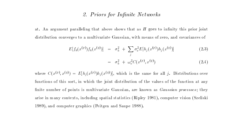
In loose terms, what Radford considers is what happens to the elements of the covariance function, \[ \begin{align*} k_f\left(\mathbf{ x}_i, \mathbf{ x}_j\right) & = \alpha \boldsymbol{ \phi}\left(\mathbf{W}_1, \mathbf{ x}_i\right)^\top \boldsymbol{ \phi}\left(\mathbf{W}_1, \mathbf{ x}_j\right)\\ & = \alpha \sum_k \phi\left(\mathbf{ w}^{(1)}_k, \mathbf{ x}_i\right) \phi\left(\mathbf{ w}^{(1)}_k, \mathbf{ x}_j\right) \end{align*} \] if instead of considering a finite number you sample infinitely many of these activation functions, sampling parameters from a prior density, \(p(\mathbf{ v})\), for each one,

\[ k_f\left(\mathbf{ x}_i, \mathbf{ x}_j\right) = \alpha \int \phi\left(\mathbf{ w}^{(1)}, \mathbf{ x}_i\right) \phi\left(\mathbf{ w}^{(1)}, \mathbf{ x}_j\right) p(\mathbf{ w}^{(1)}) \text{d}\mathbf{ w}^{(1)} \] And that’s not only for Gaussian \(p(\mathbf{ v})\). In fact this result holds for a range of activations, and a range of prior densities because of the central limit theorem.

To write it in the form of a probabilistic program, as long as the distribution for \(\phi_i\) implied by this short probabilistic program, \[ \begin{align*} \mathbf{ v}& \sim p(\cdot)\\ \phi_i & = \phi\left(\mathbf{ v}, \mathbf{ x}_i\right), \end{align*} \] has finite variance, then the result of taking the number of hidden units to infinity, with appropriate scaling, is also a Gaussian process.

Further Reading

To understand this argument in more detail, I highly recommend reading chapter 2 of Neal’s thesis (Neal, 1994), which remains easy to read and clear today. Indeed, for readers interested in Bayesian neural networks, both Raford Neal’s and David MacKay’s PhD thesis (MacKay, 1992) remain essential reading. Both theses embody a clarity of thought, and an ability to weave together threads from different fields that was the business of machine learning in the 1990s. Radford and David were also pioneers in making their software widely available and publishing material on the web.

Gaussian Process

In our we sampled from the prior over paraemters. Through the properties of multivariate Gaussian densities this prior over parameters implies a particular density for our data observations, \(\mathbf{ y}\). In this session we sampled directly from this distribution for our data, avoiding the intermediate weight-space representation. This is the approach taken by Gaussian processes. In a Gaussian process you specify the covariance function directly, rather than implicitly through a basis matrix and a prior over parameters. Gaussian processes have the advantage that they can be nonparametric, which in simple terms means that they can have infinite basis functions. In the lectures we introduced the exponentiated quadratic covariance, also known as the RBF or the Gaussian or the squared exponential covariance function. This covariance function is specified by \[ k(\mathbf{ x}, \mathbf{ x}^\prime) = \alpha \exp\left( -\frac{\left\Vert \mathbf{ x}-\mathbf{ x}^\prime\right\Vert^2}{2\ell^2}\right), \] where \(\left\Vert\mathbf{ x}- \mathbf{ x}^\prime\right\Vert^2\) is the squared distance between the two input vectors \[ \left\Vert\mathbf{ x}- \mathbf{ x}^\prime\right\Vert^2 = (\mathbf{ x}- \mathbf{ x}^\prime)^\top (\mathbf{ x}- \mathbf{ x}^\prime) \] Let’s build a covariance matrix based on this function. First we define the form of the covariance function,

from mlai import eq_cov

We can use this to compute directly the covariance for \(\mathbf{ f}\) at the points given by x_pred. Let’s define a new function K() which does this,

from mlai import Kernel

Now we can image the resulting covariance,

kernel = mlai.Kernel(function=mlai.eq_cov, variance=1., lengthscale=10.)
K = kernel.K(x_pred, x_pred)

To visualise the covariance between the points we can use the imshow function in matplotlib.

Finally, we can sample functions from the marginal likelihood.

Exercise 2

Moving Parameters Have a play with the parameters for this covariance function (the lengthscale and the variance) and see what effects the parameters have on the types of functions you observe.

Bayesian Inference by Rejection Sampling

One view of Bayesian inference is to assume we are given a mechanism for generating samples, where we assume that mechanism is representing an accurate view on the way we believe the world works.

This mechanism is known as our prior belief.

We combine our prior belief with our observations of the real world by discarding all those prior samples that are inconsistent with our observations. The likelihood defines mathematically what we mean by inconsistent with the observations. The higher the noise level in the likelihood, the looser the notion of consistent.

The samples that remain are samples from the posterior.

This approach to Bayesian inference is closely related to two sampling techniques known as rejection sampling and importance sampling. It is realized in practice in an approach known as approximate Bayesian computation (ABC) or likelihood-free inference.

In practice, the algorithm is often too slow to be practical, because most samples will be inconsistent with the observations and as a result the mechanism must be operated many times to obtain a few posterior samples.

However, in the Gaussian process case, when the likelihood also assumes Gaussian noise, we can operate this mechanism mathematically, and obtain the posterior density analytically. This is the benefit of Gaussian processes.

First, we will load in two python functions for computing the covariance function.

Next, we sample from a multivariate normal density (a multivariate Gaussian), using the covariance function as the covariance matrix.

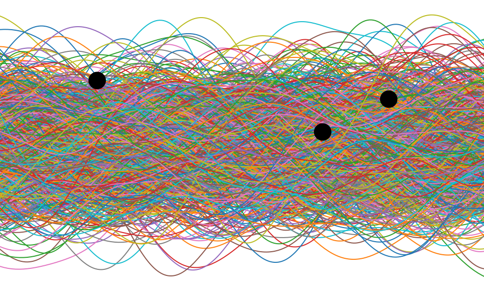
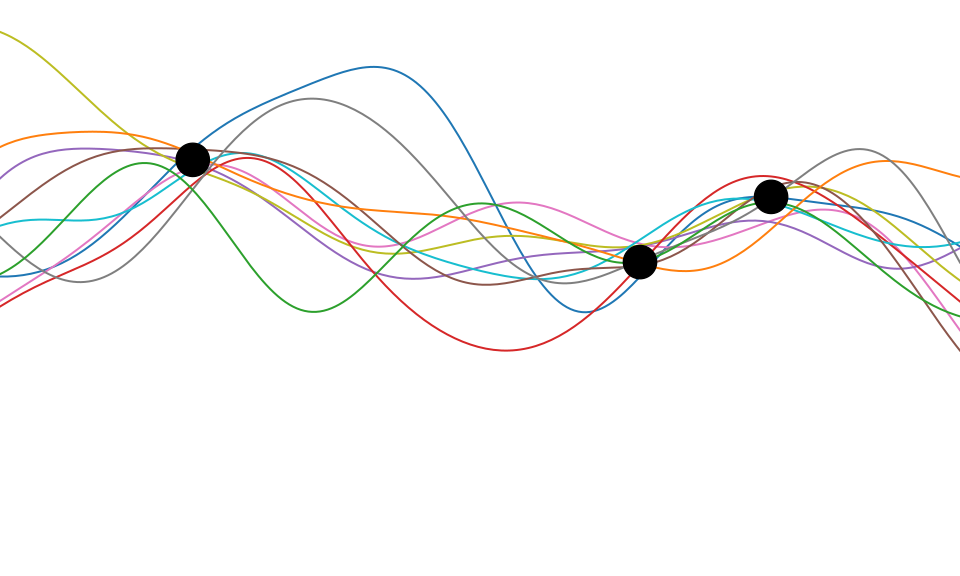
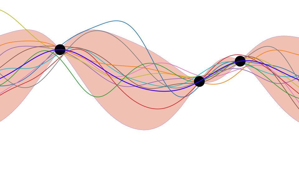
Figure: One view of Bayesian inference is we have a machine for generating samples (the prior), and we discard all samples inconsistent with our data, leaving the samples of interest (the posterior). This is a rejection sampling view of Bayesian inference. The Gaussian process allows us to do this analytically by multiplying the prior by the likelihood.

Making Predictions with Gaussian Process

The Gaussian process perspective takes the marginal likelihood of the data to be a joint Gaussian density with a covariance given by \(\mathbf{K}\). So the model likelihood is of the form, \[ p(\mathbf{ y}|\mathbf{X}) = \frac{1}{(2\pi)^{\frac{n}{2}}|\mathbf{K}|^{\frac{1}{2}}} \exp\left(-\frac{1}{2}\mathbf{ y}^\top \left(\mathbf{K}+\sigma^2 \mathbf{I}\right)^{-1}\mathbf{ y}\right) \] where the input data, \(\mathbf{X}\), influences the density through the covariance matrix, \(\mathbf{K}\) whose elements are computed through the covariance function, \(k(\mathbf{ x}, \mathbf{ x}^\prime)\).

This means that the negative log likelihood (the objective function) is given by, \[ E(\boldsymbol{\theta}) = \frac{1}{2} \log |\mathbf{K}| + \frac{1}{2} \mathbf{ y}^\top \left(\mathbf{K}+ \sigma^2\mathbf{I}\right)^{-1}\mathbf{ y} \] where the parameters of the model are also embedded in the covariance function, they include the parameters of the kernel (such as lengthscale and variance), and the noise variance, \(\sigma^2\). Let’s create a set of classes in python for storing these variables.

from mlai import ProbMapModel

from mlai import GP

Making Predictions

We now have a probability density that represents functions. How do we make predictions with this density? The density is known as a process because it is consistent. By consistency, here, we mean that the model makes predictions for \(\mathbf{ f}\) that are unaffected by future values of \(\mathbf{ f}^*\) that are currently unobserved (such as test points). If we think of \(\mathbf{ f}^*\) as test points, we can still write down a joint probability density over the training observations, \(\mathbf{ f}\) and the test observations, \(\mathbf{ f}^*\). This joint probability density will be Gaussian, with a covariance matrix given by our covariance function, \(k(\mathbf{ x}_i, \mathbf{ x}_j)\). \[ \begin{bmatrix}\mathbf{ f}\\ \mathbf{ f}^*\end{bmatrix} \sim \mathscr{N}\left(\mathbf{0},\begin{bmatrix} \mathbf{K}& \mathbf{K}_\ast \\ \mathbf{K}_\ast^\top & \mathbf{K}_{\ast,\ast}\end{bmatrix}\right) \] where here \(\mathbf{K}\) is the covariance computed between all the training points, \(\mathbf{K}_\ast\) is the covariance matrix computed between the training points and the test points and \(\mathbf{K}_{\ast,\ast}\) is the covariance matrix computed betwen all the tests points and themselves. To be clear, let’s compute these now for our example, using x and y for the training data (although y doesn’t enter the covariance) and x_pred as the test locations.

# set covariance function parameters
variance = 16.0
lengthscale = 8
# set noise variance
sigma2 = 0.05

kernel = Kernel(eq_cov, variance=variance, lengthscale=lengthscale)
K = kernel.K(x, x)
K_star = kernel.K(x, x_pred)
K_starstar = kernel.K(x_pred, x_pred)

Now we use this structure to visualise the covariance between test data and training data. This structure is how information is passed between test and training data. Unlike the maximum likelihood formalisms we’ve been considering so far, the structure expresses correlation between our different data points. However, just like the we now have a joint density between some variables of interest. In particular we have the joint density over \(p(\mathbf{ f}, \mathbf{ f}^*)\). The joint density is Gaussian and zero mean. It is specified entirely by the covariance matrix, \(\mathbf{K}\). That covariance matrix is, in turn, defined by a covariance function. Now we will visualise the form of that covariance in the form of the matrix, \[ \begin{bmatrix} \mathbf{K}& \mathbf{K}_\ast \\ \mathbf{K}_\ast^\top & \mathbf{K}_{\ast,\ast}\end{bmatrix} \]

Figure: Different blocks of the covariance function. The upper left block is the covariance of the training data with itself, \(\mathbf{K}\). The top right is the cross covariance between training data (rows) and prediction locations (columns). The lower left is the same matrix transposed. The bottom right is the covariance matrix of the test data with itself.

There are four blocks to this plot. The upper left block is the covariance of the training data with itself, \(\mathbf{K}\). We see some structure here due to the missing data from the first and second world wars. Alongside this covariance (to the right and below) we see the cross covariance between the training and the test data (\(\mathbf{K}_*\) and \(\mathbf{K}_*^\top\)). This is giving us the covariation between our training and our test data. Finally the lower right block The banded structure we now observe is because some of the training points are near to some of the test points. This is how we obtain ‘communication’ between our training data and our test data. If there is no structure in \(\mathbf{K}_*\) then our belief about the test data simply matches our prior.

Prediction Across Two Points with GPs

Sampling a Function

We will consider a multivariate Gaussian with a particular structure of covariance matrix. We will generate a single sample from this 25 dimensional Gaussian density.

\[ \mathbf{ f}=\left[f_{1},f_{2}\dots f_{25}\right]. \] in the figure below we plot these data on the \(y\)-axis against their indices on the \(x\)-axis.

import numpy as np
np.random.seed(4949)

from mlai import Kernel

from mlai import polynomial_cov

from mlai import eq_cov

Sampling a Function from a Gaussian

Figure: The joint Gaussian over \(f_1\) and \(f_2\) along with the conditional distribution of \(f_2\) given \(f_1\)

Joint Density of \(f_1\) and \(f_2\)

Figure: The joint Gaussian over \(f_1\) and \(f_2\) along with the conditional distribution of \(f_2\) given \(f_1\)

Uluru

Figure: Uluru, the sacred rock in Australia. If we think of it as a probability density, viewing it from this side gives us one marginal from the density. Figuratively speaking, slicing through the rock would give a conditional density.

When viewing these contour plots, I sometimes find it helpful to think of Uluru, the prominent rock formation in Australia. The rock rises above the surface of the plane, just like a probability density rising above the zero line. The rock is three dimensional, but when we view Uluru from the classical position, we are looking at one side of it. This is equivalent to viewing the marginal density.

The joint density can be viewed from above, using contours. The conditional density is equivalent to slicing the rock. Uluru is a holy rock, so this has to be an imaginary slice. Imagine we cut down a vertical plane orthogonal to our view point (e.g. coming across our view point). This would give a profile of the rock, which when renormalized, would give us the conditional distribution, the value of conditioning would be the location of the slice in the direction we are facing.

Prediction of \(f_2\) from \(f_1\)

Of course in practice, rather than manipulating mountains physically, the advantage of the Gaussian density is that we can perform these manipulations mathematically.

Prediction of \(f_2\) given \(f_1\) requires the conditional density, \(p(f_2|f_1)\).Another remarkable property of the Gaussian density is that this conditional distribution is also guaranteed to be a Gaussian density. It has the form, \[ p(f_2|f_1) = \mathscr{N}\left(f_2|\frac{k_{1, 2}}{k_{1, 1}}f_1, k_{2, 2} - \frac{k_{1,2}^2}{k_{1,1}}\right) \]where we have assumed that the covariance of the original joint density was given by \[ \mathbf{K}= \begin{bmatrix} k_{1, 1} & k_{1, 2}\\ k_{2, 1} & k_{2, 2}.\end{bmatrix} \]

Using these formulae we can determine the conditional density for any of the elements of our vector \(\mathbf{ f}\). For example, the variable \(f_8\) is less correlated with \(f_1\) than \(f_2\). If we consider this variable we see the conditional density is more diffuse.

Joint Density of \(f_1\) and \(f_8\)

Figure: Sample from the joint Gaussian model, points indexed by 1 and 8 highlighted.

Prediction of \(f_{8}\) from \(f_{1}\)

Figure: The joint Gaussian over \(f_1\) and \(f_8\) along with the conditional distribution of \(f_8\) given \(f_1\)

• The single contour of the Gaussian density represents the joint distribution, \(p(f_1, f_8)\)

. . .

• We observe a value for \(f_1=-?\)

. . .

• Conditional density: \(p(f_8|f_1=?)\).

• Prediction of \(\mathbf{ f}_*\) from \(\mathbf{ f}\).

• Multivariate conditional density is also Gaussian. \[ p(\mathbf{ f}_*|\mathbf{ f}) = {\mathcal{N}\left(\mathbf{ f}_*|\mathbf{K}_{*,\mathbf{ f}}\mathbf{K}_{\mathbf{ f},\mathbf{ f}}^{-1}\mathbf{ f},\mathbf{K}_{*,*}-\mathbf{K}_{*,\mathbf{ f}} \mathbf{K}_{\mathbf{ f},\mathbf{ f}}^{-1}\mathbf{K}_{\mathbf{ f},*}\right)} \]

• Here covariance of joint density is given by \[ \mathbf{K}= \begin{bmatrix} \mathbf{K}_{\mathbf{ f}, \mathbf{ f}} & \mathbf{K}_{*, \mathbf{ f}}\\ \mathbf{K}_{\mathbf{ f}, *} & \mathbf{K}_{*, *}\end{bmatrix} \]

• Prediction of \(\mathbf{ f}_*\) from \(\mathbf{ f}\).

• Multivariate conditional density is also Gaussian. \[ p(\mathbf{ f}_*|\mathbf{ f}) = {\mathcal{N}\left(\mathbf{ f}_*|\boldsymbol{ \mu},\boldsymbol{ \Sigma}\right)} \] \[ \boldsymbol{ \mu}= \mathbf{K}_{*,\mathbf{ f}}\mathbf{K}_{\mathbf{ f},\mathbf{ f}}^{-1}\mathbf{ f} \] \[ \boldsymbol{ \Sigma}= \mathbf{K}_{*,*}-\mathbf{K}_{*,\mathbf{ f}} \mathbf{K}_{\mathbf{ f},\mathbf{ f}}^{-1}\mathbf{K}_{\mathbf{ f},*} \]

• Here covariance of joint density is given by \[ \mathbf{K}= \begin{bmatrix} \mathbf{K}_{\mathbf{ f}, \mathbf{ f}} & \mathbf{K}_{*, \mathbf{ f}}\\ \mathbf{K}_{\mathbf{ f}, *} & \mathbf{K}_{*, *}\end{bmatrix} \]

The Importance of the Covariance Function

The covariance function encapsulates our assumptions about the data. The equations for the distribution of the prediction function, given the training observations, are highly sensitive to the covariation between the test locations and the training locations as expressed by the matrix \(\mathbf{K}_*\). We defined a matrix \(\mathbf{A}\) which allowed us to express our conditional mean in the form, \[ \boldsymbol{ \mu}_f= \mathbf{A}^\top \mathbf{ y}, \] where \(\mathbf{ y}\) were our training observations. In other words our mean predictions are always a linear weighted combination of our training data. The weights are given by computing the covariation between the training and the test data (\(\mathbf{K}_*\)) and scaling it by the inverse covariance of the training data observations, \(\left[\mathbf{K}+ \sigma^2 \mathbf{I}\right]^{-1}\). This inverse is the main computational object that needs to be resolved for a Gaussian process. It has a computational burden which is \(O(n^3)\) and a storage burden which is \(O(n^2)\). This makes working with Gaussian processes computationally intensive for the situation where \(n>10,000\).

Figure: Introduction to Gaussian processes given by Neil Lawrence at the 2014 Gaussian process Winter School at the University of Sheffield.

Improving the Numerics

In practice we shouldn’t be using matrix inverse directly to solve the GP system. One more stable way is to compute the Cholesky decomposition of the kernel matrix. The log determinant of the covariance can also be derived from the Cholesky decomposition.

import scipy.linalg as la

from mlai import GP

from mlai import update_inverse

# Bind the updated inverse to our GP model
GP.update_inverse = update_inverse

Capacity Control

Gaussian processes are sometimes seen as part of a wider family of methods known as kernel methods. Kernel methods are also based around covariance functions, but in the field they are known as Mercer kernels. Mercer kernels have interpretations as inner products in potentially infinite dimensional Hilbert spaces. This interpretation arises because, if we take \(\alpha=1\), then the kernel can be expressed as \[ \mathbf{K}= \boldsymbol{ \Phi}\boldsymbol{ \Phi}^\top \] which imples the elements of the kernel are given by, \[ k(\mathbf{ x}, \mathbf{ x}^\prime) = \boldsymbol{ \phi}(\mathbf{ x})^\top \boldsymbol{ \phi}(\mathbf{ x}^\prime). \] So we see that the kernel function is developed from an inner product between the basis functions. Mercer’s theorem tells us that any valid positive definite function can be expressed as this inner product but with the caveat that the inner product could be infinite length. This idea has been used quite widely to kernelize algorithms that depend on inner products. The kernel functions are equivalent to covariance functions and they are parameterized accordingly. In the kernel modeling community it is generally accepted that kernel parameter estimation is a difficult problem and the normal solution is to cross validate to obtain parameters. This can cause difficulties when a large number of kernel parameters need to be estimated. In Gaussian process modelling kernel parameter estimation (in the simplest case proceeds) by maximum likelihood. This involves taking gradients of the likelihood with respect to the parameters of the covariance function.

Gradients of the Likelihood

The easiest conceptual way to obtain the gradients is a two step process. The first step involves taking the gradient of the likelihood with respect to the covariance function, the second step involves considering the gradient of the covariance function with respect to its parameters.

Overall Process Scale

In general we won’t be able to find parameters of the covariance function through fixed point equations, we will need to do gradient based optimization.

Capacity Control and Data Fit

The objective function can be decomposed into two terms, a capacity control term, and a data fit term. The capacity control term is the log determinant of the covariance. The data fit term is the matrix inner product between the data and the inverse covariance.

Learning Covariance Parameters

Can we determine covariance parameters from the data?

\[ \mathscr{N}\left(\mathbf{ y}|\mathbf{0},\mathbf{K}\right)=\frac{1}{(2\pi)^\frac{n}{2}{\det{\mathbf{K}}^{\frac{1}{2}}}}{\exp\left(-\frac{\mathbf{ y}^{\top}\mathbf{K}^{-1}\mathbf{ y}}{2}\right)} \]

\[ \begin{aligned} \mathscr{N}\left(\mathbf{ y}|\mathbf{0},\mathbf{K}\right)=\frac{1}{(2\pi)^\frac{n}{2}\color{blue}{\det{\mathbf{K}}^{\frac{1}{2}}}}\color{red}{\exp\left(-\frac{\mathbf{ y}^{\top}\mathbf{K}^{-1}\mathbf{ y}}{2}\right)} \end{aligned} \]

\[ \begin{aligned} \log \mathscr{N}\left(\mathbf{ y}|\mathbf{0},\mathbf{K}\right)=&\color{blue}{-\frac{1}{2}\log\det{\mathbf{K}}}\color{red}{-\frac{\mathbf{ y}^{\top}\mathbf{K}^{-1}\mathbf{ y}}{2}} \\ &-\frac{n}{2}\log2\pi \end{aligned} \]

\[ E(\boldsymbol{ \theta}) = \color{blue}{\frac{1}{2}\log\det{\mathbf{K}}} + \color{red}{\frac{\mathbf{ y}^{\top}\mathbf{K}^{-1}\mathbf{ y}}{2}} \]

Capacity Control through the Determinant

The parameters are inside the covariance function (matrix). \[k_{i, j} = k(\mathbf{ x}_i, \mathbf{ x}_j; \boldsymbol{ \theta})\]

\[\mathbf{K}= \mathbf{R}\boldsymbol{ \Lambda}^2 \mathbf{R}^\top\]

\(\boldsymbol{ \Lambda}\) represents distance on axes. \(\mathbf{R}\) gives rotation.

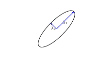
• \(\boldsymbol{ \Lambda}\) is diagonal, \(\mathbf{R}^\top\mathbf{R}= \mathbf{I}\).
• Useful representation since \(\det{\mathbf{K}} = \det{\boldsymbol{ \Lambda}^2} = \det{\boldsymbol{ \Lambda}}^2\).

Figure: The determinant of the covariance is dependent only on the eigenvalues. It represents the ‘footprint’ of the Gaussian.

Quadratic Data Fit

Figure: The data fit term of the Gaussian process is a quadratic loss centered around zero. This has eliptical contours, the principal axes of which are given by the covariance matrix.

Data Fit Term

x = np.linspace(-1, 1, 6)[:, np.newaxis]
xtest = np.linspace(x_lim[0], x_lim[1], 200)[:, np.newaxis]

# True data
true_kernel = Kernel(eq_cov, name='Exponentiated Quadratic', shortname='eq', lengthscale=1)
K = true_kernel.K(x) + np.eye(6)*0.01 
y = np.random.multivariate_normal(np.zeros((6,)), K, 1).T

# Fitted model
kernel = Kernel(eq_cov, name='Exponentiated Quadratic', shortname='eq', lengthscale=1)
gp = GP(x, y, sigma2=0.01, kernel=kernel)

Figure: Variation in the data fit term, the capacity term and the negative log likelihood for different lengthscales.

Exponentiated Quadratic Covariance

The exponentiated quadratic covariance, also known as the Gaussian covariance or the RBF covariance and the squared exponential. Covariance between two points is related to the negative exponential of the squared distnace between those points. This covariance function can be derived in a few different ways: as the infinite limit of a radial basis function neural network, as diffusion in the heat equation, as a Gaussian filter in Fourier space or as the composition as a series of linear filters applied to a base function.

The covariance takes the following form, \[ k(\mathbf{ x}, \mathbf{ x}^\prime) = \alpha \exp\left(-\frac{\left\Vert \mathbf{ x}-\mathbf{ x}^\prime \right\Vert_2^2}{2\ell^2}\right) \] where \(\ell\) is the length scale or time scale of the process and \(\alpha\) represents the overall process variance.

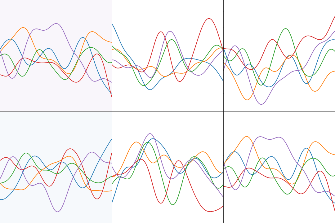
Figure: The exponentiated quadratic covariance function.

GPSS: Gaussian Process Summer School

If you’re interested in finding out more about Gaussian processes, you can attend the Gaussian process summer school, or view the lectures and material on line. Details of the school, future events and past events can be found at the website http://gpss.cc.

cmd = install_command('GPy')

%system {cmd}

GPy: A Gaussian Process Framework in Python

Gaussian processes are a flexible tool for non-parametric analysis with uncertainty. The GPy software was started in Sheffield to provide a easy to use interface to GPs. One which allowed the user to focus on the modelling rather than the mathematics.

Figure: GPy is a BSD licensed software code base for implementing Gaussian process models in Python. It is designed for teaching and modelling. We welcome contributions which can be made through the GitHub repository https://github.com/SheffieldML/GPy

GPy is a BSD licensed software code base for implementing Gaussian process models in python. This allows GPs to be combined with a wide variety of software libraries.

The software itself is available on GitHub and the team welcomes contributions.

The aim for GPy is to be a probabilistic-style programming language, i.e., you specify the model rather than the algorithm. As well as a large range of covariance functions the software allows for non-Gaussian likelihoods, multivariate outputs, dimensionality reduction and approximations for larger data sets.

The documentation for GPy can be found here.

GPy Tutorial

This GPy tutorial is based on material we share in the Gaussian process summer school for teaching these models https://gpss.cc. It contains material from various members and former members of the Sheffield machine learning group, but particular mention should be made of Nicolas Durrande and James Hensman, see http://gpss.cc/gpss17/labs/GPSS_Lab1_2017.ipynb.

cmd = install_command('GPy')

%system {cmd}

cmd = install_command('mlai')

%system {cmd}

import numpy as np
import GPy

To give a feel for the software we’ll start by creating an exponentiated quadratic covariance function, \[ k(\mathbf{ x}, \mathbf{ x}^\prime) = \alpha \exp\left(-\frac{\left\Vert \mathbf{ x}- \mathbf{ x}^\prime \right\Vert_2^2}{2\ell^2}\right), \] where the length scale is \(\ell\) and the variance is \(\alpha\).

To set this up in GPy we create a kernel in the following manner.

input_dim=1
alpha = 1.0
lengthscale = 2.0
kern = GPy.kern.RBF(input_dim=input_dim, variance=alpha, lengthscale=lengthscale)

That builds a kernel object for us. The kernel can be displayed.

display(kern)

Or because it’s one dimensional, you can also plot the kernel as a function of its inputs (while the other is fixed).

Figure: The exponentiated quadratic covariance function as plotted by the GPy.kern.plot command.

You can set the length scale of the covariance to different values and plot the result.

kern = GPy.kern.RBF(input_dim=input_dim)     # By default, the parameters are set to 1.
lengthscales = np.asarray([0.2,0.5,1.,2.,4.])

Figure: The exponentiated quadratic covariance function plotted for different length scales by GPy.kern.plot command.

Covariance Functions in GPy

Many covariance functions are already implemented in GPy. Instead of rbf, try constructing and plotting the following covariance functions: exponential, Matern32, Matern52, Brownian, linear, bias, rbfcos, periodic_Matern32, etc. Some of these covariance functions, such as rbfcos, are not parametrized by a variance and a length scale. Further, not all kernels are stationary (i.e., they can’t all be written as \(k(\mathbf{ x}, \mathbf{ x}^\prime) = f(\mathbf{ x}-\mathbf{ x}^\prime)\), see for example the Brownian covariance function). So for plotting it may be interesting to change the value of the fixed input.

Combining Covariance Functions in GPy

In GPy you can easily combine covariance functions you have created using the sum and product operators, + and *. So, for example, if we wish to combine an exponentiated quadratic covariance with a Matern 5/2 then we can write

kern1 = GPy.kern.RBF(1, variance=1., lengthscale=2.)
kern2 = GPy.kern.Matern52(1, variance=2., lengthscale=4.)
kern = kern1 + kern2
display(kern)

Figure: A combination of the exponentiated quadratic covariance plus the Matern \(5/2\) covariance.

Or if we wanted to multiply them, we can write

kern1 = GPy.kern.RBF(1, variance=1., lengthscale=2.)
kern2 = GPy.kern.Matern52(1, variance=2., lengthscale=4.)
kern = kern1 * kern2
display(kern)

Figure: A combination of the exponentiated quadratic covariance multiplied by the Matern \(5/2\) covariance.

You can learn about how to implement new kernel objects in GPy here.

Figure: Designing the covariance function for your Gaussian process is a key place in which you introduce your understanding of the data problem. To learn more about the design of covariance functions, see this talk from Nicolas Durrande at GPSS in 2016.

A Gaussian Process Regression Model

We will now combine the Gaussian process prior with some data to form a GP regression model with GPy. We will generate data from the function \[ f( x) = − \cos(\pi x) + \sin(4\pi x) \] over the domain \([0, 1]\), adding some noise to gives \[ y(x) = f(x) + \epsilon, \] with the noise being Gaussian distributed, \(\epsilon\sim \mathscr{N}\left(0,0.01\right)\).

X = np.linspace(0.05,0.95,10)[:,np.newaxis]
Y = -np.cos(np.pi*X) + np.sin(4*np.pi*X) + np.random.normal(loc=0.0, scale=0.1, size=(10,1))

Figure: Data from the noisy sine wave for fitting with a GPy model.

A GP regression model based on an exponentiated quadratic covariance function can be defined by first defining a covariance function.

kern = GPy.kern.RBF(input_dim=1, variance=1., lengthscale=1.)

And then combining it with the data to form a Gaussian process model.

model = GPy.models.GPRegression(X,Y,kern)

Just as for the covariance function object, we can find out about the model using the command display(model).

display(model)

Note that by default the model includes some observation noise with variance 1. We can see the posterior mean prediction and visualize the marginal posterior variances using model.plot().

Figure: A Gaussian process fit to the noisy sine data. Here the parameters of the process and the covariance function haven’t yet been optimized.

You can also look directly at the predictions for the model using.

Xstar = np.linspace(0, 10, 100)[:, np.newaxis]
Ystar, Vstar = model.predict(Xstar)

Which gives you the mean (Ystar), the variance (Vstar) at the locations given by Xstar.

Covariance Function Parameter Estimation

As we have seen during the lectures, the parameters values can be estimated by maximizing the likelihood of the observations. Since we don’t want any of the variances to become negative during the optimization, we can constrain all parameters to be positive before running the optimization.

model.constrain_positive()

The warnings are because the parameters are already constrained by default, the software is warning us that they are being reconstrained.

Now we can optimize the model using the model.optimize() method. Here we switch messages on, which allows us to see the progression of the optimization.

model.optimize(messages=True)

By default, the optimization is using a limited memory BFGS optimizer (Byrd et al., 1995).

Once again, we can display the model, now to see how the parameters have changed.

display(model)

The length scale is much smaller, as well as the noise level. The variance of the exponentiated quadratic has also reduced.

Figure: A Gaussian process fit to the noisy sine data with parameters optimized.

Review

Other Software

GPy has inspired other software solutions, first of all GPflow, which uses Tensor Flow’s automatic differentiation engine to allow rapid prototyping of new covariance functions and algorithms. More recently, GPyTorch uses PyTorch for the same purpose.

The Probabilistic programming language pyro also has GP support.

Further Reading

• Chapter 2 of Neal (1994)

• Rest of Neal (1994)

• All of MacKay (1992)

Thanks!

For more information on these subjects and more you might want to check the following resources.

• company: Trent AI
• book: The Atomic Human
• twitter: @lawrennd
• podcast: The Talking Machines
• newspaper: Guardian Profile Page
• blog: http://inverseprobability.com

References