Gaussian Processes

A First Course in Machine Learning

Example: Prediction of Malaria Incidence in Uganda

• Work with Ricardo Andrade Pacheco, John Quinn and Martin Mubangizi (Makerere University, Uganda)
• See AI-DEV Group.
• See UN Global Pulse Disease Outbreaks Site

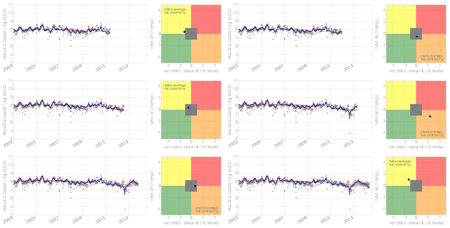
Malaria Prediction in Uganda

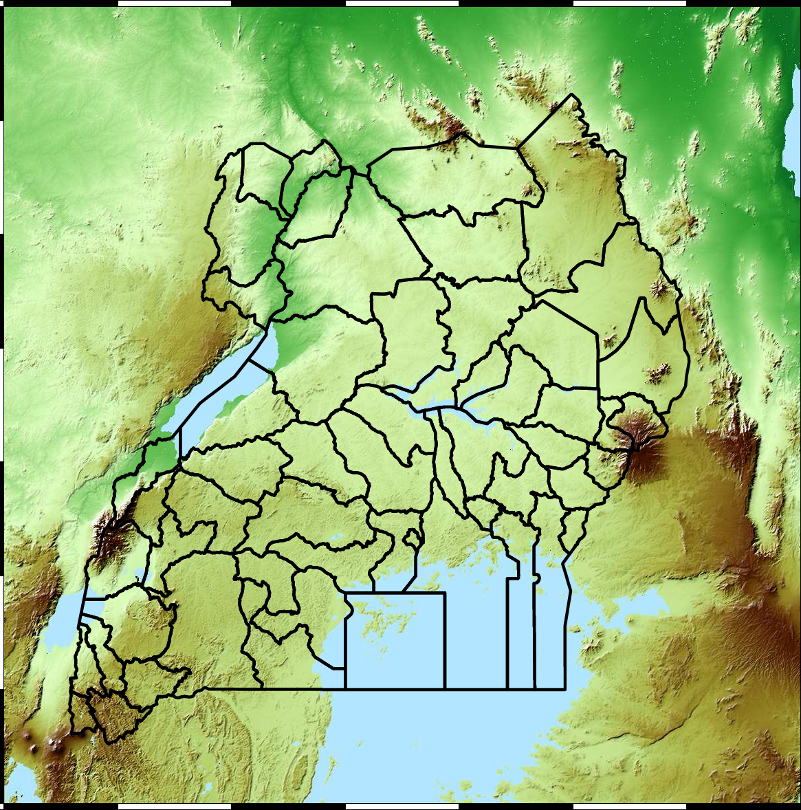
Tororo District

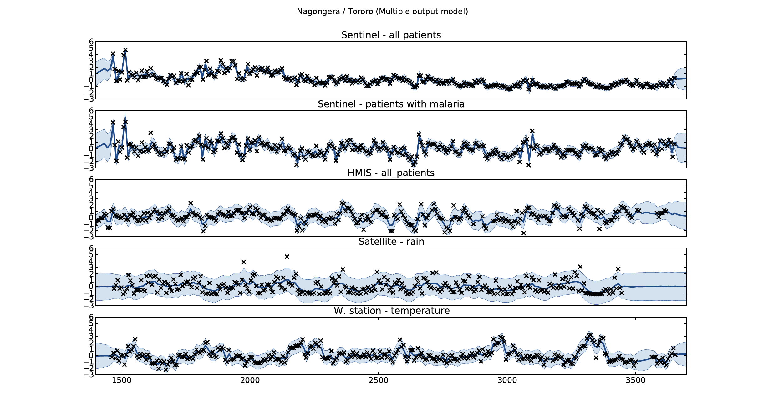
Malaria Prediction in Nagongera (Sentinel Site)

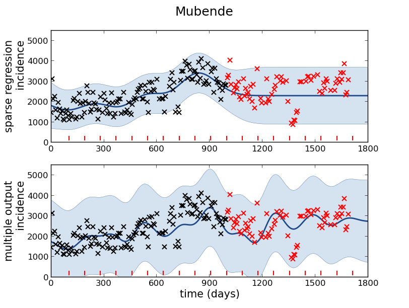
Mubende District

Malaria Prediction in Uganda

GP School at Makerere

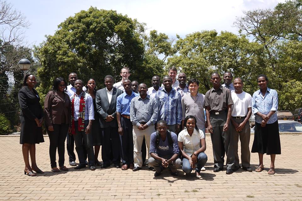
Kabarole District

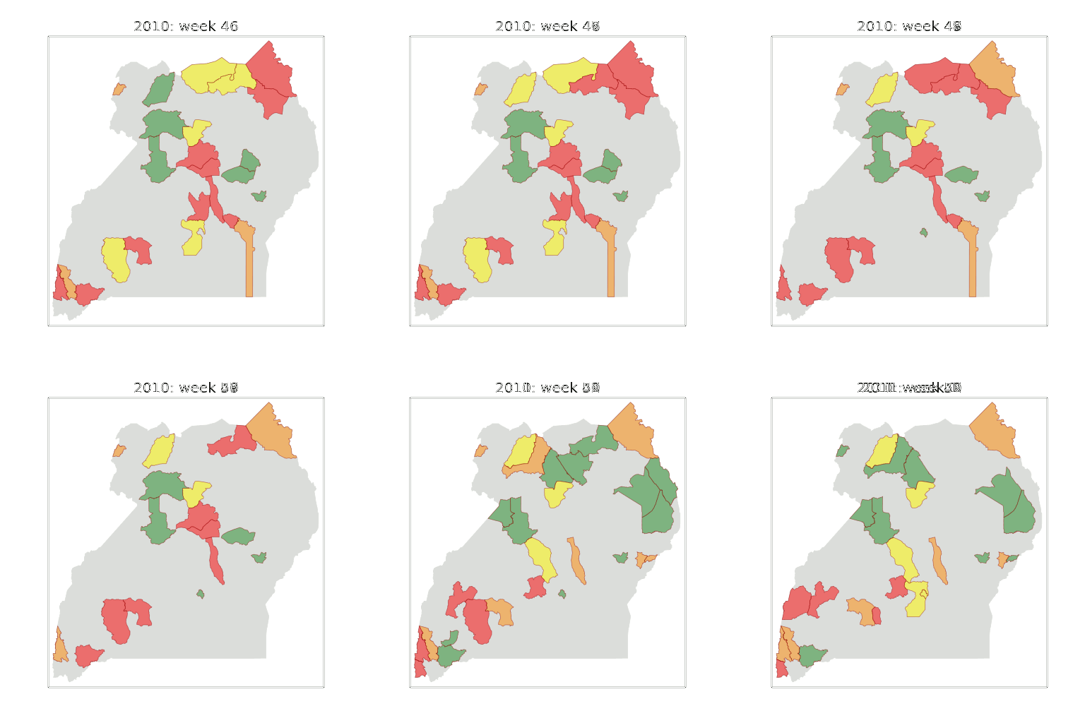
Early Warning System

Early Warning Systems

What is Machine Learning?

What is Machine Learning?

What is Machine Learning?

\[\text{data} + \text{model} \stackrel{\text{compute}}{\rightarrow} \text{prediction}\]

• To combine data with a model need:
• a prediction function \(f(\cdot)\) includes our beliefs about the regularities of the universe
• an objective function \(E(\cdot)\) defines the cost of misprediction.

Overdetermined System

\(y= mx+ c\)

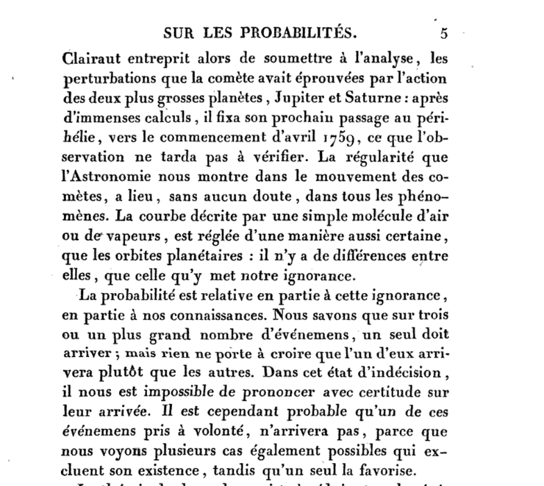
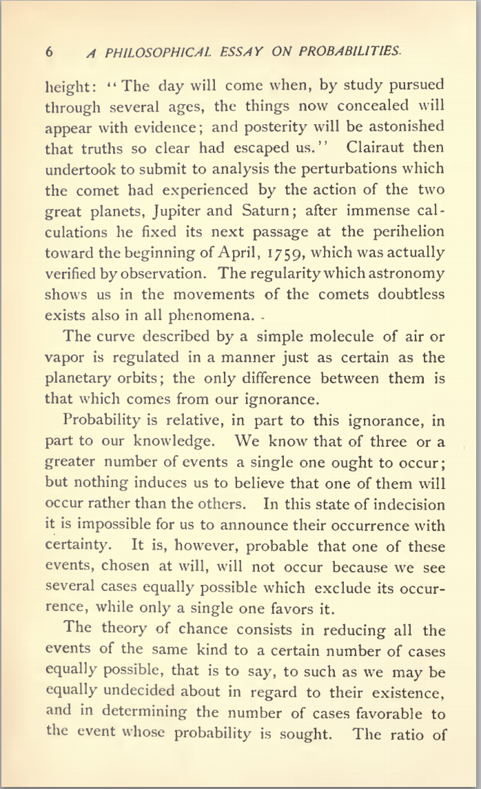
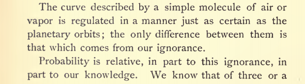
Pierre-Simon Laplace

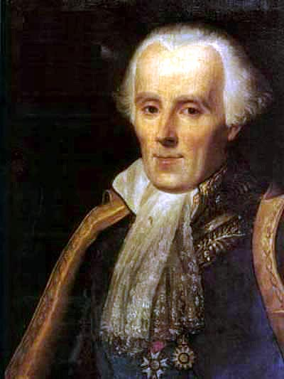
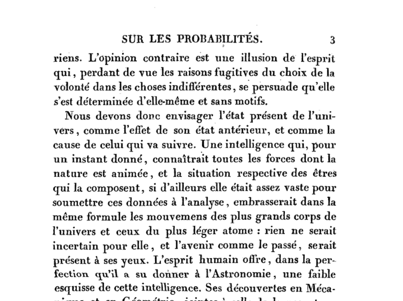
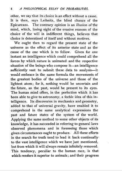
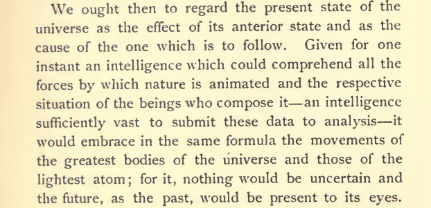
Laplace’s Gremlin

Latent Variables

\(y= mx+ c + \epsilon\)

A Probabilistic Process

Two Important Gaussian Properties

Sum of Gaussians

Scaling a Gaussian

Multivariate Gaussian Properties

• If \[ \mathbf{ y}= \mathbf{W}\mathbf{ x}+ \boldsymbol{ \epsilon}, \]

• Assume \[ \begin{align} \mathbf{ x}& \sim \mathscr{N}\left(\boldsymbol{ \mu},\mathbf{C}\right)\\ \boldsymbol{ \epsilon}& \sim \mathscr{N}\left(\mathbf{0},\boldsymbol{ \Sigma}\right) \end{align} \]

• Then \[ \mathbf{ y}\sim \mathscr{N}\left(\mathbf{W}\boldsymbol{ \mu},\mathbf{W}\mathbf{C}\mathbf{W}^\top + \boldsymbol{ \Sigma}\right). \] If \(\boldsymbol{ \Sigma}=\sigma^2\mathbf{I}\), this is Probabilistic PCA (Tipping and Bishop, 1999).

Objective Optimization

Multivariate Derivatives

• We will need some multivariate calculus.
• For now some simple multivariate differentiation: \[\frac{\text{d}{\mathbf{a}^{\top}}{\mathbf{ w}}}{\text{d}\mathbf{ w}}=\mathbf{a}\] and \[\frac{\mathbf{ w}^{\top}\mathbf{A}\mathbf{ w}}{\text{d}\mathbf{ w}}=\left(\mathbf{A}+\mathbf{A}^{\top}\right)\mathbf{ w}\] or if \(\mathbf{A}\) is symmetric (i.e. \(\mathbf{A}=\mathbf{A}^{\top}\)) \[\frac{\text{d}\mathbf{ w}^{\top}\mathbf{A}\mathbf{ w}}{\text{d}\mathbf{ w}}=2\mathbf{A}\mathbf{ w}.\]

Differentiate the Objective

\[ \frac{\partial L\left(\mathbf{ w},\sigma^2 \right)}{\partial \mathbf{ w}}=\frac{1}{\sigma^2} \sum _{i=1}^{n}\mathbf{ x}_i y_i-\frac{1}{\sigma^2} \left[\sum _{i=1}^{n}\mathbf{ x}_i\mathbf{ x}_i^{\top}\right]\mathbf{ w} \] Leading to \[ \mathbf{ w}^{*}=\left[\sum _{i=1}^{n}\mathbf{ x}_i\mathbf{ x}_i^{\top}\right]^{-1}\sum _{i=1}^{n}\mathbf{ x}_iy_i, \]

Differentiate the Objective

Rewrite in matrix notation: \[ \sum_{i=1}^{n}\mathbf{ x}_i\mathbf{ x}_i^\top = \boldsymbol{ \Phi}^\top \boldsymbol{ \Phi} \] \[ \sum_{i=1}^{n}\mathbf{ x}_iy_i = \boldsymbol{ \Phi}^\top \mathbf{ y} \]

Update Equation for Global Optimum

Update Equations

• Solve the matrix equation for \(\mathbf{ w}\). \[\boldsymbol{ \Phi}^\top \boldsymbol{ \Phi}\mathbf{ w}= \boldsymbol{ \Phi}^\top \mathbf{ y}\]

• The equation for \(\left.\sigma^2\right.^{*}\) may also be found \[\left.\sigma^2\right.^{{*}}=\frac{\sum_{i=1}^{n}\left(y_i-\left.\mathbf{ w}^{*}\right.^{\top}\mathbf{ x}_i\right)^{2}}{n}.\]

Movie Violence Data

• Data containing movie information (year, length, rating, genre, IMDB Rating).
• Try and predict what factors influence a movie’s violence

Multivariate Regression on Movie Violence Data

• Regress from features Year, Body_Count, Length_Minutes to IMDB_Rating.

Residuals

Underdetermined System

Underdetermined System

• What about two unknowns and one observation? \[y_1 = mx_1 + c\]

Underdetermined System

Two Dimensional Gaussian

• Consider height, \(h/m\) and weight, \(w/kg\).
• Could sample height from a distribution: \[ p(h) \sim \mathscr{N}\left(1.7,0.0225\right). \]
• And similarly weight: \[ p(w) \sim \mathscr{N}\left(75,36\right). \]

Height and Weight Models

Independence Assumption

• We assume height and weight are independent.

  \[ p(w, h) = p(w)p(h). \]

Sampling Two Dimensional Variables

displaycode{nu.display_plots(‘independent_height_weight{fig:0>3}.svg’, directory=‘./ml’, fig=IntSlider(0, 0, 7, 1))}

Body Mass Index

• In reality they are dependent (body mass index) \(= \frac{w}{h^2}\).
• To deal with this dependence we introduce correlated multivariate Gaussians.

Sampling Two Dimensional Variables

Independent Gaussians

\[ p(w, h) = p(w)p(h) \]

Independent Gaussians

Independent Gaussians

\[ p(w, h) = \frac{1}{\sqrt{2\pi\sigma_1^22\pi\sigma_2^2}} \exp\left(-\frac{1}{2}\left(\begin{bmatrix}w \\ h\end{bmatrix} - \begin{bmatrix}\mu_1 \\ \mu_2\end{bmatrix}\right)^\top\begin{bmatrix}\sigma_1^2& 0\\0&\sigma_2^2\end{bmatrix}^{-1}\left(\begin{bmatrix}w \\ h\end{bmatrix} - \begin{bmatrix}\mu_1 \\ \mu_2\end{bmatrix}\right)\right) \]

Independent Gaussians

\[ p(\mathbf{ y}) = \frac{1}{\det{2\pi \mathbf{D}}^{\frac{1}{2}}} \exp\left(-\frac{1}{2}(\mathbf{ y}- \boldsymbol{ \mu})^\top\mathbf{D}^{-1}(\mathbf{ y}- \boldsymbol{ \mu})\right) \]

Correlated Gaussian

\[ p(\mathbf{ y}) = \frac{1}{\det{2\pi\mathbf{D}}^{\frac{1}{2}}} \exp\left(-\frac{1}{2}(\mathbf{ y}- \boldsymbol{ \mu})^\top\mathbf{D}^{-1}(\mathbf{ y}- \boldsymbol{ \mu})\right) \]

Correlated Gaussian

\[ p(\mathbf{ y}) = \frac{1}{\det{2\pi\mathbf{D}}^{\frac{1}{2}}} \exp\left(-\frac{1}{2}(\mathbf{R}^\top\mathbf{ y}- \mathbf{R}^\top\boldsymbol{ \mu})^\top\mathbf{D}^{-1}(\mathbf{R}^\top\mathbf{ y}- \mathbf{R}^\top\boldsymbol{ \mu})\right) \]

Correlated Gaussian

\[ p(\mathbf{ y}) = \frac{1}{\det{2\pi\mathbf{D}}^{\frac{1}{2}}} \exp\left(-\frac{1}{2}(\mathbf{ y}- \boldsymbol{ \mu})^\top\mathbf{R}\mathbf{D}^{-1}\mathbf{R}^\top(\mathbf{ y}- \boldsymbol{ \mu})\right) \]

\[ \mathbf{C}^{-1} = \mathbf{R}\mathbf{D}^{-1} \mathbf{R}^\top \]

Correlated Gaussian

\[ p(\mathbf{ y}) = \frac{1}{\det{2\pi\mathbf{C}}^{\frac{1}{2}}} \exp\left(-\frac{1}{2}(\mathbf{ y}- \boldsymbol{ \mu})^\top\mathbf{C}^{-1} (\mathbf{ y}- \boldsymbol{ \mu})\right) \] \[ \mathbf{C}= \mathbf{R}\mathbf{D} \mathbf{R}^\top \]

Basis Functions

Quadratic Basis

• Basis functions can be global. E.g. quadratic basis: \[ \boldsymbol{ \phi}= [1, x, x^2] \]

\[ \begin{align*} \phi_1(x) & = 1, \\ \phi_2(x) & = x, \\ \phi_3(x) & = x^2. \end{align*} \]

\[ \boldsymbol{ \phi}(x) = \begin{bmatrix} 1\\ x \\ x^2\end{bmatrix}. \]

Matrix Valued Function

\[ \boldsymbol{ \Phi}(\mathbf{ x}) = \begin{bmatrix} 1 & x_1 & x_1^2 \\ 1 & x_2 & x_2^2\\ \vdots & \vdots & \vdots \\ 1 & x_n & x_n^2 \end{bmatrix} \]

Functions Derived from Quadratic Basis

\[ f(x) = {\color{cyan}{w_0}} + {\color{green}{w_1 x}} + {\color{yellow}{w_2 x^2}} \]

Quadratic Functions

\[ f(x) = {\color{cyan}{w_0}} + {\color{green}{w_1 x}} + {\color{yellow}{w_2 x^2}} \]

Rectified Linear Units

• The ReLU is a basis function used in neural nets

\[ \phi_j(x) = xH(x+ v_j) \]

Functions Derived from Relu Basis

\[ f(x) = \color{cyan}{w_0} + \color{green}{w_1 xH(x+1.0) } + \color{yellow}{w_2 xH(x+0.33) } + \color{magenta}{w_3 xH(x-0.33)} + \color{red}{w_4 xH(x-1.0)} \]

Gaussian Processes

• Basis function models give non-linear predictions.
• Need to choose number and location of basis functions.
• Gaussian processes is a general framework (basis functions special case)
• Within the framework you can consider models with infinite basis functions.

\[ p(\mathbf{ y}|\mathbf{X}, \mathbf{ w}) = \prod_{i=1}^{n} p(y_i | \mathbf{ x}_i, \mathbf{ w}) \]

\[ \mathbf{ y}|\mathbf{X}\sim \mathscr{N}\left(\mathbf{m}(\mathbf{X}),\mathbf{K}(\mathbf{X})\right), \]

Linear Model Overview

• Set each activation function computed at each data point to be

\[ \phi_{i,j} = \phi(\mathbf{ w}^{(1)}_{j}, \mathbf{ x}_{i}) \] Define design matrix \[ \boldsymbol{ \Phi}= \begin{bmatrix} \phi_{1, 1} & \phi_{1, 2} & \dots & \phi_{1, h} \\ \phi_{1, 2} & \phi_{1, 2} & \dots & \phi_{1, n} \\ \vdots & \vdots & \ddots & \vdots \\ \phi_{n, 1} & \phi_{n, 2} & \dots & \phi_{n, h} \end{bmatrix}. \]

Matrix Representation of a Neural Network

\[y\left(\mathbf{ x}\right) = \boldsymbol{ \phi}\left(\mathbf{ x}\right)^\top \mathbf{ w}+ \epsilon\]

Multivariate Gaussian Properties

• If \[ \mathbf{ y}= \mathbf{W}\mathbf{ x}+ \boldsymbol{ \epsilon}, \]

• Assume \[ \begin{align} \mathbf{ x}& \sim \mathscr{N}\left(\boldsymbol{ \mu},\mathbf{C}\right)\\ \boldsymbol{ \epsilon}& \sim \mathscr{N}\left(\mathbf{0},\boldsymbol{ \Sigma}\right) \end{align} \]

• Then \[ \mathbf{ y}\sim \mathscr{N}\left(\mathbf{W}\boldsymbol{ \mu},\mathbf{W}\mathbf{C}\mathbf{W}^\top + \boldsymbol{ \Sigma}\right). \] If \(\boldsymbol{ \Sigma}=\sigma^2\mathbf{I}\), this is Probabilistic PCA (Tipping and Bishop, 1999).

Prior Density

• Define \[ \mathbf{ w}\sim \mathscr{N}\left(\mathbf{0},\alpha\mathbf{I}\right), \]
• Rules of multivariate Gaussians to see that, \[ \mathbf{ y}\sim \mathscr{N}\left(\mathbf{0},\alpha \boldsymbol{ \Phi}\boldsymbol{ \Phi}^\top + \sigma^2 \mathbf{I}\right). \]

\[ \mathbf{K}= \alpha \boldsymbol{ \Phi}\boldsymbol{ \Phi}^\top + \sigma^2 \mathbf{I}. \]

Joint Gaussian Density

• Elements are a function \(k_{i,j} = k\left(\mathbf{ x}_i, \mathbf{ x}_j\right)\)

\[ \mathbf{K}= \alpha \boldsymbol{ \Phi}\boldsymbol{ \Phi}^\top + \sigma^2 \mathbf{I}. \]

Covariance Function

\[ k_f\left(\mathbf{ x}_i, \mathbf{ x}_j\right) = \alpha \boldsymbol{ \phi}\left(\mathbf{W}_1, \mathbf{ x}_i\right)^\top \boldsymbol{ \phi}\left(\mathbf{W}_1, \mathbf{ x}_j\right) \]

• formed by inner products of the rows of the design matrix.

Gaussian Process

• Instead of making assumptions about our density over each data point, \(y_i\) as i.i.d.

• make a joint Gaussian assumption over our data.

• covariance matrix is now a function of both the parameters of the activation function, \(\mathbf{W}_1\), and the input variables, \(\mathbf{X}\).

• Arises from integrating out \(\mathbf{ w}^{(2)}\).

Basis Functions

• Can be very complex, such as deep kernels, (Cho and Saul, 2009) or could even put a convolutional neural network inside.
• Viewing a neural network in this way is also what allows us to beform sensible batch normalizations (Ioffe and Szegedy, 2015).

Radial Basis Functions

• Basis functions can be local e.g. radial (or Gaussian) basis \[ \phi_j(x) = \exp\left(-\frac{(x-\mu_j)^2}{\ell^2}\right) \]

Radial Basis Functions

Functions Derived from Radial Basis

\[ f(x) = \color{cyan}{w_1 e^{-2(x+1)^2}} + \color{green}{w_2e^{-2x^2}} + \color{yellow}{w_3 e^{-2(x-1)^2}} \]

Marginal Likelihood

• Build on our understanding of marginal likelihood.

Generating from the Model

\[ \mathbf{ y}= \boldsymbol{ \Phi}\mathbf{ w}+ \boldsymbol{ \epsilon} \]

• Sample \[ \mathbf{ w}\sim \mathscr{N}\left(0,\alpha\mathbf{I}\right) \] \[ \boldsymbol{ \epsilon}\sim \mathscr{N}\left(\mathbf{0},\sigma^2\right) \] with \(\alpha=1\) and \(\sigma^2 = 0.01\).

Olympic Marathon Polynomial Sample

Sampling from the Prior

K = degree + 1
z_vec = np.random.normal(size=K)
w_sample = z_vec*np.sqrt(alpha)

f_sample = Phi_pred@w_sample

Mean Output

• Each sample \(\mathbf{ w}_s\) has a prediction \(\mathbf{ f}_s\)

\[ \mathbf{ f}_s = \boldsymbol{ \Phi}\mathbf{ w}_s. \]

for i in range(num_samples):
    z_vec = np.random.normal(size=K)
    w_sample = z_vec*np.sqrt(alpha)
    f_sample = np.dot(Phi_pred,w_sample)
    _ = ax.plot(x_pred.flatten(), f_sample.flatten(), linewidth=2)

Function Space View

\[ \mathbf{ w}\sim \mathscr{N}\left(\mathbf{0},\alpha \mathbf{I}\right) \] \[ \boldsymbol{ \Phi}= \begin{bmatrix}\boldsymbol{ \phi}(\mathbf{ x}_1) \\ \vdots \\ \boldsymbol{ \phi}(\mathbf{ x}_n)\end{bmatrix} \] \[ \mathbf{ f}= \begin{bmatrix} f_1 \\ \vdots \\ f_n\end{bmatrix} \] \[ \mathbf{ f}= \boldsymbol{ \Phi}\mathbf{ w}. \]

\[ \mathbf{ f}\sim \mathscr{N}\left(\mathbf{0},\alpha \boldsymbol{ \Phi}\boldsymbol{ \Phi}^\top\right). \]

\[ \mathbf{K}= \alpha \boldsymbol{ \Phi}\boldsymbol{ \Phi}^\top. \]

K = alpha*Phi_pred@Phi_pred.T

K = alpha*Phi_pred@Phi_pred.T f_sample = np.random.multivariate_normal(mean=np.zeros(x_pred.size), cov=K)

\[ \mathbf{ y}= \mathbf{ f}+ \boldsymbol{\epsilon} \]

\[ \epsilon \sim \mathscr{N}\left(\mathbf{0},\sigma^2\mathbf{I}\right). \]

\[ \mathbf{ y}\sim \mathscr{N}\left(\mathbf{0},\boldsymbol{ \Phi}\boldsymbol{ \Phi}^\top +\sigma^2\mathbf{I}\right). \]

Non-degenerate Gaussian Processes

• This process is degenerate.
• Covariance function is of rank at most \(h\).
• As \(n\rightarrow \infty\), covariance matrix is not full rank.
• Leading to \(\det{\mathbf{K}} = 0\)

Infinite Networks

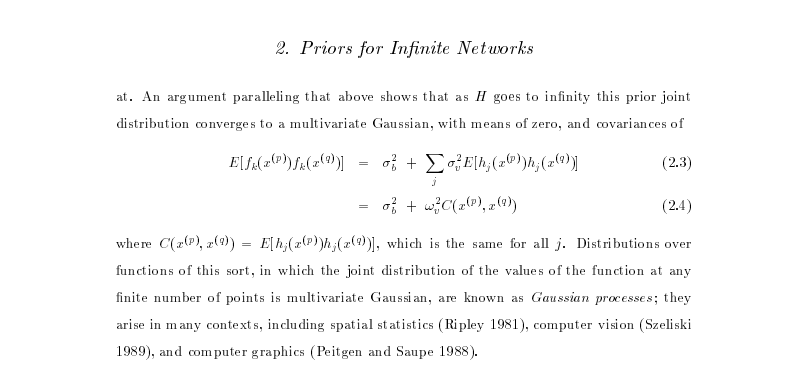
• In ML Radford Neal (Neal, 1994) asked “what would happen if you took \(h\rightarrow \infty\)?”

Roughly Speaking

• Instead of \[ \begin{align*} k_f\left(\mathbf{ x}_i, \mathbf{ x}_j\right) & = \alpha \boldsymbol{ \phi}\left(\mathbf{W}_1, \mathbf{ x}_i\right)^\top \boldsymbol{ \phi}\left(\mathbf{W}_1, \mathbf{ x}_j\right)\\ & = \alpha \sum_k \phi\left(\mathbf{ w}^{(1)}_k, \mathbf{ x}_i\right) \phi\left(\mathbf{ w}^{(1)}_k, \mathbf{ x}_j\right) \end{align*} \]

• Sample infinitely many from a prior density, \(p(\mathbf{ w}^{(1)})\), \[ k_f\left(\mathbf{ x}_i, \mathbf{ x}_j\right) = \alpha \int \phi\left(\mathbf{ w}^{(1)}, \mathbf{ x}_i\right) \phi\left(\mathbf{ w}^{(1)}, \mathbf{ x}_j\right) p(\mathbf{ w}^{(1)}) \text{d}\mathbf{ w}^{(1)} \]
• Also applies for non-Gaussian \(p(\mathbf{ w}^{(1)})\) because of the central limit theorem.

Simple Probabilistic Program

• If \[ \begin{align*} \mathbf{ w}^{(1)} & \sim p(\cdot)\\ \phi_i & = \phi\left(\mathbf{ w}^{(1)}, \mathbf{ x}_i\right), \end{align*} \] has finite variance.

• Then taking number of hidden units to infinity, is also a Gaussian process.

Further Reading

• Chapter 2 of Neal’s thesis (Neal, 1994)

• Rest of Neal’s thesis. (Neal, 1994)

• David MacKay’s PhD thesis (MacKay, 1992)

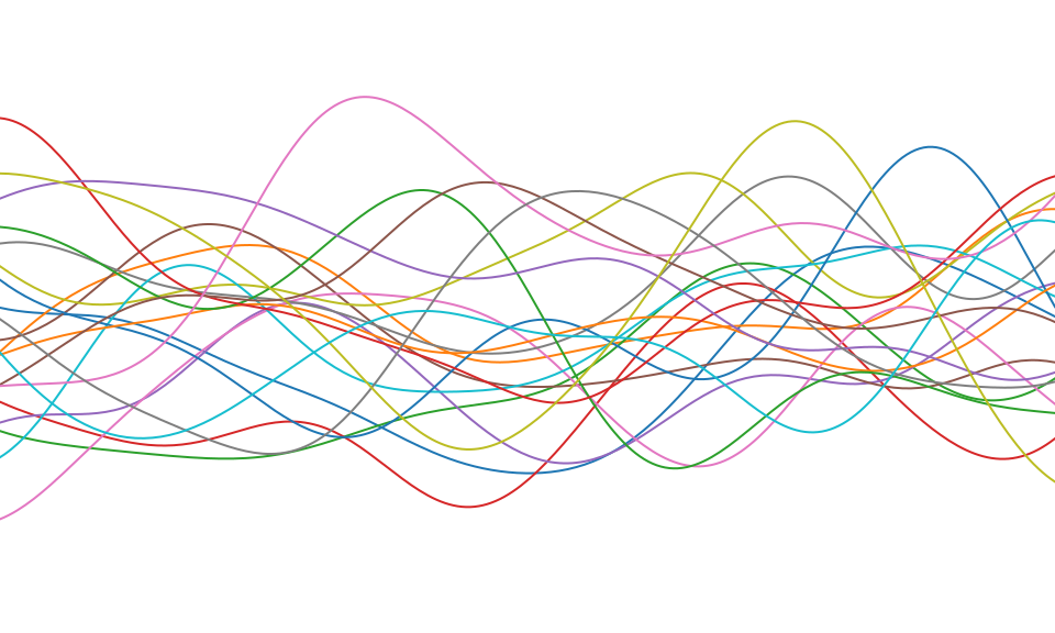
Gaussian Process

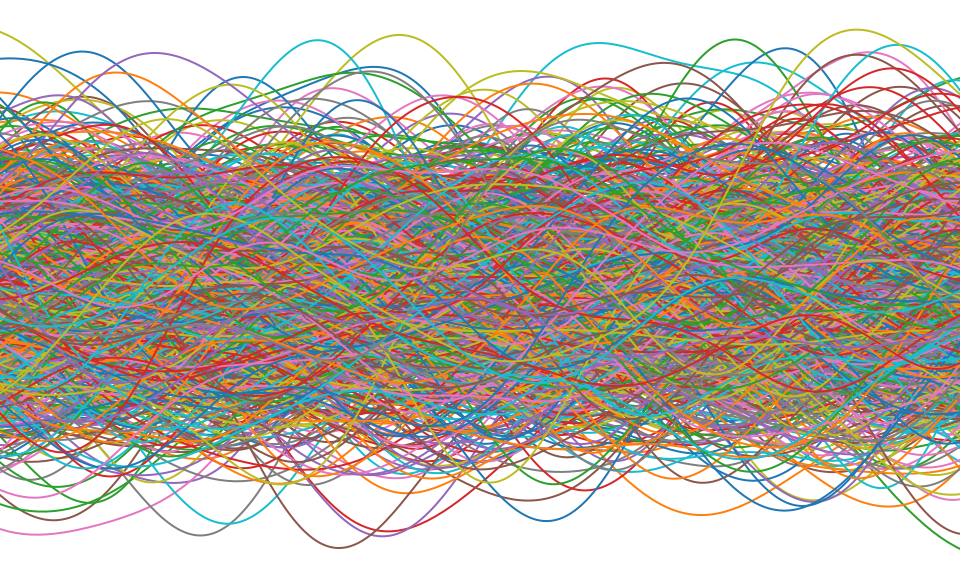
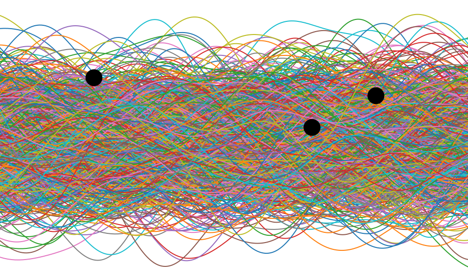
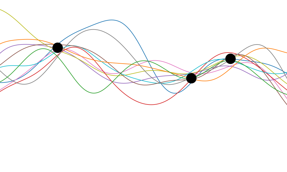
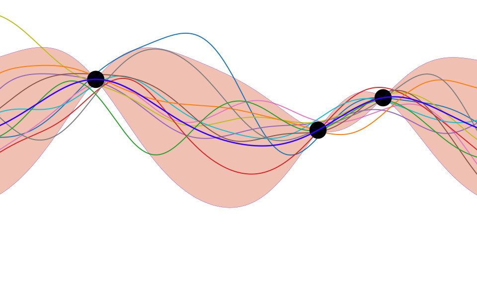
\[ k(\mathbf{ x}, \mathbf{ x}^\prime) = \alpha \exp\left( -\frac{\left\Vert \mathbf{ x}-\mathbf{ x}^\prime\right\Vert^2}{2\ell^2}\right), \]

\[ \left\Vert\mathbf{ x}- \mathbf{ x}^\prime\right\Vert^2 = (\mathbf{ x}- \mathbf{ x}^\prime)^\top (\mathbf{ x}- \mathbf{ x}^\prime) \]

Making Predictions with Gaussian Process

\[ p(\mathbf{ y}|\mathbf{X}) = \frac{1}{(2\pi)^{\frac{n}{2}}|\mathbf{K}|^{\frac{1}{2}}} \exp\left(-\frac{1}{2}\mathbf{ y}^\top \left(\mathbf{K}+\sigma^2 \mathbf{I}\right)^{-1}\mathbf{ y}\right) \]

\[ E(\boldsymbol{\theta}) = \frac{1}{2} \log |\mathbf{K}| + \frac{1}{2} \mathbf{ y}^\top \left(\mathbf{K}+ \sigma^2\mathbf{I}\right)^{-1}\mathbf{ y} \]

Making Predictions

\[ \begin{bmatrix}\mathbf{ f}\\ \mathbf{ f}^*\end{bmatrix} \sim \mathscr{N}\left(\mathbf{0},\begin{bmatrix} \mathbf{K}& \mathbf{K}_\ast \\ \mathbf{K}_\ast^\top & \mathbf{K}_{\ast,\ast}\end{bmatrix}\right) \]

\[ \begin{bmatrix} \mathbf{K}& \mathbf{K}_\ast \\ \mathbf{K}_\ast^\top & \mathbf{K}_{\ast,\ast}\end{bmatrix} \]

Making Predictions

Sampling a Function

Multi-variate Gaussians

• We will consider a Gaussian with a particular structure of covariance matrix.
• Generate a single sample from this 25 dimensional Gaussian density, \[ \mathbf{ f}=\left[f_{1},f_{2}\dots f_{25}\right]. \]
• We will plot these points against their index.

Sampling a Function from a Gaussian

Joint Density of \(f_1\) and \(f_2\)

Prediction of \(f_{2}\) from \(f_{1}\)

Uluru

Prediction of \(f_2\) from \(f_1\)

• Conditional density is also Gaussian. \[ p(f_2|f_1) = \mathscr{N}\left(f_2|\frac{k_{1, 2}}{k_{1, 1}}f_1, k_{2, 2} - \frac{k_{1,2}^2}{k_{1,1}}\right) \] where covariance of joint density is given by \[ \mathbf{K}= \begin{bmatrix} k_{1, 1} & k_{1, 2}\\ k_{2, 1} & k_{2, 2}.\end{bmatrix} \]

Joint Density of \(f_1\) and \(f_8\)

Prediction of \(f_{8}\) from \(f_{1}\)

Details

• The single contour of the Gaussian density represents the joint distribution, \(p(f_1, f_8)\)

Multivariate Conditional Density

• Prediction of \(\mathbf{ f}_*\) from \(\mathbf{ f}\).

• Multivariate conditional density is also Gaussian. \[ p(\mathbf{ f}_*|\mathbf{ f}) = {\mathcal{N}\left(\mathbf{ f}_*|\mathbf{K}_{*,\mathbf{ f}}\mathbf{K}_{\mathbf{ f},\mathbf{ f}}^{-1}\mathbf{ f},\mathbf{K}_{*,*}-\mathbf{K}_{*,\mathbf{ f}} \mathbf{K}_{\mathbf{ f},\mathbf{ f}}^{-1}\mathbf{K}_{\mathbf{ f},*}\right)} \]

• Here covariance of joint density is given by \[ \mathbf{K}= \begin{bmatrix} \mathbf{K}_{\mathbf{ f}, \mathbf{ f}} & \mathbf{K}_{*, \mathbf{ f}}\\ \mathbf{K}_{\mathbf{ f}, *} & \mathbf{K}_{*, *}\end{bmatrix} \]

Multivariate Conditional Density

• Prediction of \(\mathbf{ f}_*\) from \(\mathbf{ f}\).

• Multivariate conditional density is also Gaussian. \[ p(\mathbf{ f}_*|\mathbf{ f}) = {\mathcal{N}\left(\mathbf{ f}_*|\boldsymbol{ \mu},\boldsymbol{ \Sigma}\right)} \] \[ \boldsymbol{ \mu}= \mathbf{K}_{*,\mathbf{ f}}\mathbf{K}_{\mathbf{ f},\mathbf{ f}}^{-1}\mathbf{ f} \] \[ \boldsymbol{ \Sigma}= \mathbf{K}_{*,*}-\mathbf{K}_{*,\mathbf{ f}} \mathbf{K}_{\mathbf{ f},\mathbf{ f}}^{-1}\mathbf{K}_{\mathbf{ f},*} \]

Prediction with Correlated Gaussians

• Here covariance of joint density is given by \[ \mathbf{K}= \begin{bmatrix} \mathbf{K}_{\mathbf{ f}, \mathbf{ f}} & \mathbf{K}_{*, \mathbf{ f}}\\ \mathbf{K}_{\mathbf{ f}, *} & \mathbf{K}_{*, *}\end{bmatrix} \]

The Importance of the Covariance Function

\[ \boldsymbol{ \mu}_f= \mathbf{A}^\top \mathbf{ y}, \]

Improving the Numerics

In practice we shouldn’t be using matrix inverse directly to solve the GP system. One more stable way is to compute the Cholesky decomposition of the kernel matrix. The log determinant of the covariance can also be derived from the Cholesky decomposition.

Capacity Control

Gradients of the Likelihood

Overall Process Scale

Capacity Control and Data Fit

Learning Covariance Parameters

Can we determine covariance parameters from the data?

\[ \mathscr{N}\left(\mathbf{ y}|\mathbf{0},\mathbf{K}\right)=\frac{1}{(2\pi)^\frac{n}{2}{\det{\mathbf{K}}^{\frac{1}{2}}}}{\exp\left(-\frac{\mathbf{ y}^{\top}\mathbf{K}^{-1}\mathbf{ y}}{2}\right)} \]

\[ \begin{aligned} \mathscr{N}\left(\mathbf{ y}|\mathbf{0},\mathbf{K}\right)=\frac{1}{(2\pi)^\frac{n}{2}\color{yellow}{\det{\mathbf{K}}^{\frac{1}{2}}}}\color{cyan}{\exp\left(-\frac{\mathbf{ y}^{\top}\mathbf{K}^{-1}\mathbf{ y}}{2}\right)} \end{aligned} \]

\[ \begin{aligned} \log \mathscr{N}\left(\mathbf{ y}|\mathbf{0},\mathbf{K}\right)=&\color{yellow}{-\frac{1}{2}\log\det{\mathbf{K}}}\color{cyan}{-\frac{\mathbf{ y}^{\top}\mathbf{K}^{-1}\mathbf{ y}}{2}} \\ &-\frac{n}{2}\log2\pi \end{aligned} \]

\[ E(\boldsymbol{ \theta}) = \color{yellow}{\frac{1}{2}\log\det{\mathbf{K}}} + \color{cyan}{\frac{\mathbf{ y}^{\top}\mathbf{K}^{-1}\mathbf{ y}}{2}} \]

Capacity Control through the Determinant

The parameters are inside the covariance function (matrix). \[k_{i, j} = k(\mathbf{ x}_i, \mathbf{ x}_j; \boldsymbol{ \theta})\]

Eigendecomposition of Covariance

\[\mathbf{K}= \mathbf{R}\boldsymbol{ \Lambda}^2 \mathbf{R}^\top\]

\(\boldsymbol{ \Lambda}\) represents distance on axes. \(\mathbf{R}\) gives rotation.

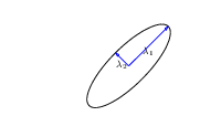
Eigendecomposition of Covariance

• \(\boldsymbol{ \Lambda}\) is diagonal, \(\mathbf{R}^\top\mathbf{R}= \mathbf{I}\).
• Useful representation since \(\det{\mathbf{K}} = \det{\boldsymbol{ \Lambda}^2} = \det{\boldsymbol{ \Lambda}}^2\).

Capacity control: \(\color{yellow}{\log \det{\mathbf{K}}}\)

Quadratic Data Fit

Data Fit: \(\color{cyan}{\frac{\mathbf{ y}^\top\mathbf{K}^{-1}\mathbf{ y}}{2}}\)

\[E(\boldsymbol{ \theta}) = \color{yellow}{\frac{1}{2}\log\det{\mathbf{K}}}+\color{cyan}{\frac{\mathbf{ y}^{\top}\mathbf{K}^{-1}\mathbf{ y}}{2}}\]

Data Fit Term

Exponentiated Quadratic Covariance

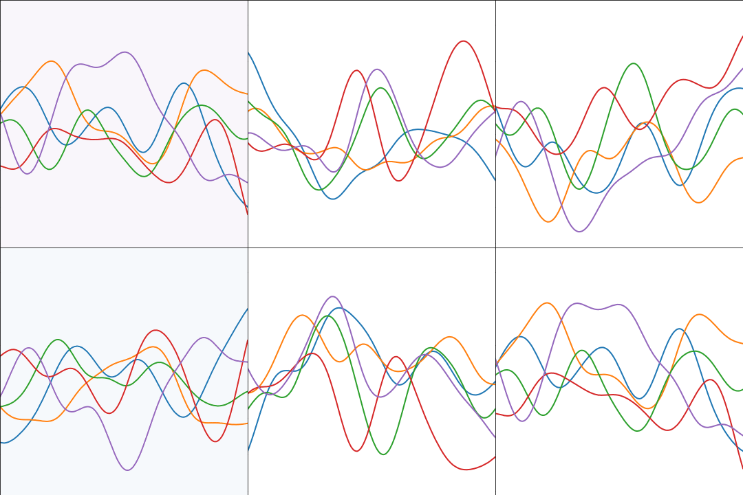
GPSS: Gaussian Process Summer School

GPy: A Gaussian Process Framework in Python

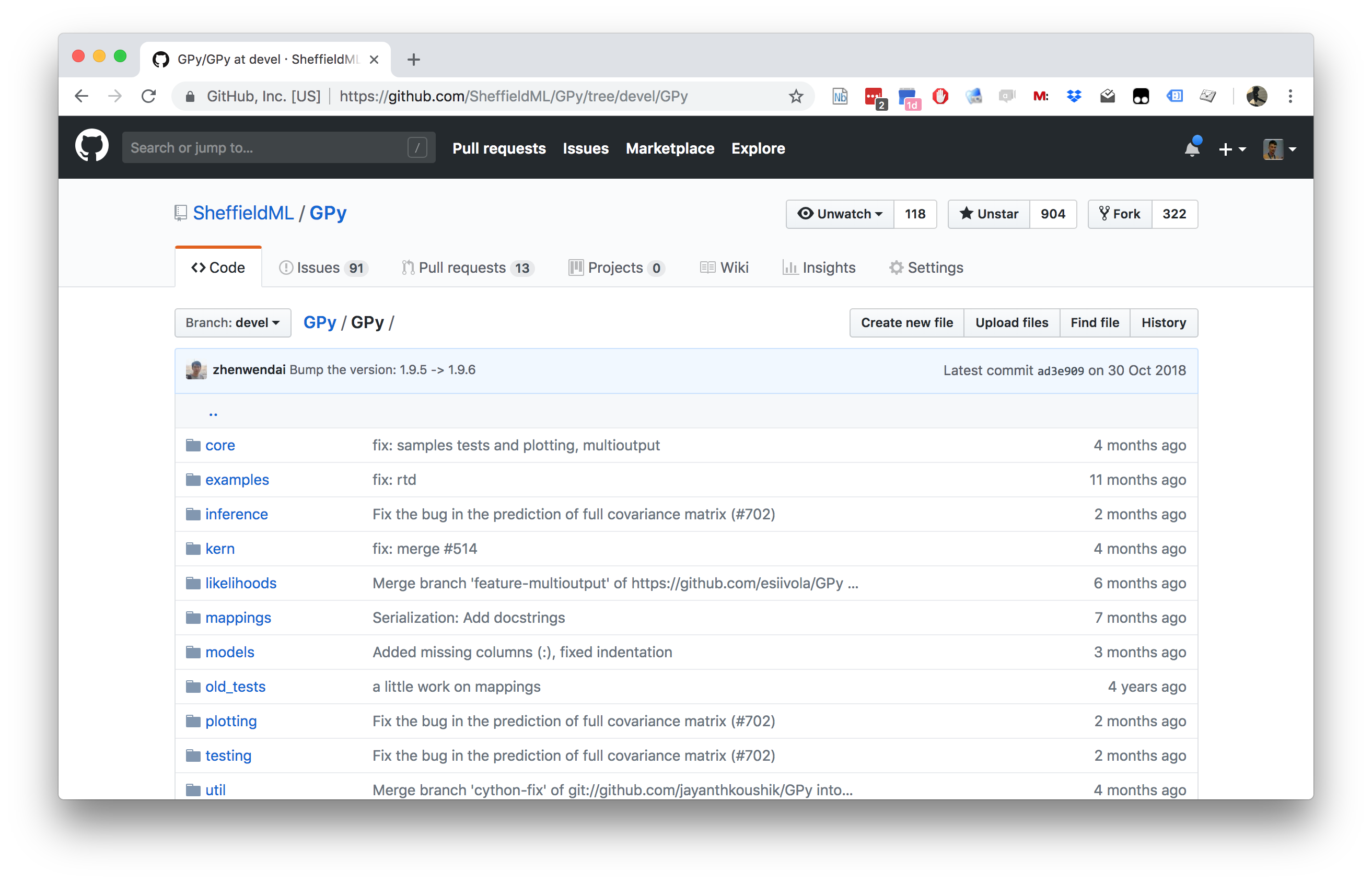
GPy: A Gaussian Process Framework in Python

• BSD Licensed software base.
• Wide availability of libraries, ‘modern’ scripting language.
• Allows us to set projects to undergraduates in Comp Sci that use GPs.
• Available through GitHub https://github.com/SheffieldML/GPy
• Reproducible Research with Jupyter Notebook.

Features

• Probabilistic-style programming (specify the model, not the algorithm).
• Non-Gaussian likelihoods.
• Multivariate outputs.
• Dimensionality reduction.
• Approximations for large data sets.

GPy Tutorial

Covariance Functions

\[ k(\mathbf{ x}, \mathbf{ x}^\prime) = \alpha \exp\left(-\frac{\left\Vert \mathbf{ x}- \mathbf{ x}^\prime \right\Vert_2^2}{2\ell^2}\right), \]

input_dim=1
alpha = 1.0
lengthscale = 2.0
kern = GPy.kern.RBF(input_dim=input_dim, 
                    variance=alpha, 
                    lengthscale=lengthscale)

Kernel Output

Covariance Functions in GPy

• Includes a range of covariance functions
  • E.g. Matern family, Brownian motion, periodic, linear etc.
  • Can define new covariances

Combining Covariance Functions in GPy

kern1 = GPy.kern.RBF(1, variance=1., lengthscale=2.)
kern2 = GPy.kern.Matern52(1, variance=2., lengthscale=4.)
kern = kern1 + kern2

Multiplication

kern1 = GPy.kern.RBF(1, variance=1., lengthscale=2.)
kern2 = GPy.kern.Matern52(1, variance=2., lengthscale=4.)
kern = kern1 * kern2
display(kern)

A Gaussian Process Regression Model

\[ f( x) = − \cos(\pi x) + \sin(4\pi x) \]

\[ y(x) = f(x) + \epsilon, \]

Noisy Sine

kern = GPy.kern.RBF(input_dim=1, variance=1., lengthscale=1.)
model = GPy.models.GPRegression(X,Y,kern)

GP Fit to Noisy Sine

Covariance Function Parameter Estimation

model.optimize(messages=True)

Review

Other Software

• GPflow
• GPyTorch
• PyRo