Week 1: Generalization and Neural Networks

[Powerpoint][jupyter][google colab][reveal][slides]

Neil D. Lawrence

Abstract:

This lecture will cover generalization in machine learning with a particular focus on neural architectures. We will review classical generalization and explore what’s different about neural network models.

Background Material

• Linear Algebra and Linear Regression by Neil D. Lawrence
• Basis Functions by Neil D. Lawrence
• Generalization: Model Validation by Neil D. Lawrence

Setup

First we download some libraries and files to support the notebook.

pods

In Sheffield we created a suite of software tools for ‘Open Data Science’. Open data science is an approach to sharing code, models and data that should make it easier for companies, health professionals and scientists to gain access to data science techniques.

You can also check this blog post on Open Data Science.

The software can be installed using

%pip install pods

from the command prompt where you can access your python installation.

The code is also available on GitHub: https://github.com/lawrennd/ods

Once pods is installed, it can be imported in the usual manner.

import pods

notutils

This small package is a helper package for various notebook utilities used below.

The software can be installed using

%pip install notutils

from the command prompt where you can access your python installation.

The code is also available on GitHub: https://github.com/lawrennd/notutils

Once notutils is installed, it can be imported in the usual manner.

import notutils

mlai

The mlai software is a suite of helper functions for teaching and demonstrating machine learning algorithms. It was first used in the Machine Learning and Adaptive Intelligence course in Sheffield in 2013.

The software can be installed using

%pip install mlai

from the command prompt where you can access your python installation.

The code is also available on GitHub: https://github.com/lawrennd/mlai

Once mlai is installed, it can be imported in the usual manner.

import mlai

Quadratic Loss and Linear System

We will consider a simplified system, to remind us of some of the linear algebra involved, and introduce some of the fundamental issues.

Expected Loss

Our objective function so far has been the negative log likelihood, which we have minimized (via the sum of squares error) to obtain our model. However, there is an alternative perspective on an objective function, that of a loss function. A loss function is a cost function associated with the penalty you might need to pay for a particular incorrect decision. One approach to machine learning involves specifying a loss function and considering how much a particular model is likely to cost us across its lifetime. We can represent this with an expectation. If our loss function is given as \(L(y, x, \mathbf{ w})\) for a particular model that predicts \(y\) given \(x\) and \(\mathbf{ w}\) then we are interested in minimizing the expected loss under the likely distribution of \(y\) and \(x\). To understand this formally we define the true distribution of the data samples, \(y\), \(x\). This is a particular distribution that we don’t typically have access to. To represent it we define a variant of the letter ‘P’, \(\mathbb{P}(y, x)\). If we genuinely pay \(L(y, x, \mathbf{ w})\) for every mistake we make, and the future test data is genuinely drawn from \(\mathbb{P}(y, x)\) then we can define our expected loss, or risk, to be, \[ R(\mathbf{ w}) = \int L(y, x, \mathbf{ w}) \mathbb{P}(y, x) \text{d}y \text{d}x. \] Of course, in practice, this value can’t be computed but it serves as a reminder of what it is we are aiming to minimize and under certain circumstances it can be approximated.

Sample-Based Approximations

A sample-based approximation to an expectation involves replacing the true expectation with a sum over samples from the distribution. \[ \int f(z) p(z) \text{d}z\approx \frac{1}{s}\sum_{i=1}^s f(z_i). \] if \(\{z_i\}_{i=1}^s\) are a set of \(s\) independent and identically distributed samples from the distribution \(p(z)\). This approximation becomes better for larger \(s\), although the rate of convergence to the true integral will be very dependent on the distribution \(p(z)\) and the function \(f(z)\).

That said, this means we can approximate our true integral with the sum, \[ R(\mathbf{ w}) \approx \frac{1}{n}\sum_{i=1}^{n} L(y_i, x_i, \mathbf{ w}). \]

Laplace’s Idea

Laplace had the idea to augment the observations by noise, that is equivalent to considering a probability density whose mean is given by the prediction function \[p\left(y_i|x_i\right)=\frac{1}{\sqrt{2\pi\sigma^2}}\exp\left(-\frac{\left(y_i-f\left(x_i\right)\right)^{2}}{2\sigma^2}\right).\]

This is known as stochastic process. It is a function that is corrupted by noise. Laplace didn’t suggest the Gaussian density for that purpose, that was an innovation from Carl Friederich Gauss, which is what gives the Gaussian density its name.

Height as a Function of Weight

In the standard Gaussian, parameterized by mean and variance, make the mean a linear function of an input.

This leads to a regression model. \[ \begin{align*} y_i=&f\left(x_i\right)+\epsilon_i,\\ \epsilon_i \sim & \mathcal{N}\left(0,\sigma^2\right). \end{align*} \]

Assume \(y_i\) is height and \(x_i\) is weight.

Olympic Marathon Data

Gold medal times for Olympic Marathon since 1896. Marathons before 1924 didn’t have a standardized distance. Present results using pace per km. In 1904 Marathon was badly organized leading to very slow times.

Image from Wikimedia Commons http://bit.ly/16kMKHQ

The first thing we will do is load a standard data set for regression modelling. The data consists of the pace of Olympic Gold Medal Marathon winners for the Olympics from 1896 to present. Let’s load in the data and plot.

import numpy as np
import pods

data = pods.datasets.olympic_marathon_men()
x = data['X']
y = data['Y']

offset = y.mean()
scale = np.sqrt(y.var())
yhat = (y - offset)/scale

Figure: Olympic marathon pace times since 1896.

Things to notice about the data include the outlier in 1904, in that year the Olympics was in St Louis, USA. Organizational problems and challenges with dust kicked up by the cars following the race meant that participants got lost, and only very few participants completed. More recent years see more consistently quick marathons.

Running Example: Olympic Marathons

Note that x and y are not pandas data frames for this example, they are just arrays of dimensionality \(n\times 1\), where \(n\) is the number of data.

The aim of this lab is to have you coding linear regression in python. We will do it in two ways, once using iterative updates (coordinate ascent) and then using linear algebra. The linear algebra approach will not only work much better, it is also easy to extend to multiple input linear regression and non-linear regression using basis functions.

Maximum Likelihood: Iterative Solution

Now we will take the maximum likelihood approach we derived in the lecture to fit a line, \(y_i=mx_i + c\), to the data you’ve plotted. We are trying to minimize the error function: \[ L(m, c) = \sum_{i=1}^n(y_i-mx_i-c)^2 \] with respect to \(m\), \(c\) and \(\sigma^2\). We can start with an initial guess for \(m\),

m = -0.4
c = 80

Then we use the maximum likelihood update to find an estimate for the offset, \(c\).

Quadratic Loss

Now we’ve identified the empirical risk with the loss, we’ll use \(L(\mathbf{ w})\) to represent our objective function. \[ L(\mathbf{ w}) = \sum_{i=1}^n\left(y_i - f(\mathbf{ x}_i, \mathbf{ w})\right)^2 \] gives us our objective.

In the case of the linear prediction function, we can substitute \(f(\mathbf{ x}_i, \mathbf{ w}) = \mathbf{ w}^\top \mathbf{ x}_i\). \[ L(\mathbf{ w}) = \sum_{i=1}^n\left(y_i - \mathbf{ w}^\top \mathbf{ x}_i\right)^2 \] To compute the gradient of the objective, we first expand the brackets.

Bracket Expansion

\[ \begin{align*} L(\mathbf{ w},\sigma^2) = & \sum _{i=1}^{n}y_i^{2}- 2\sum _{i=1}^{n}y_i\mathbf{ w}^{\top}\mathbf{ x}_i\\&+\sum _{i=1}^{n}\mathbf{ w}^{\top}\mathbf{ x}_i\mathbf{ x}_i^{\top}\mathbf{ w}\\ = & \sum_{i=1}^{n}y_i^{2}- 2 \mathbf{ w}^\top\sum_{i=1}^{n}\mathbf{ x}_iy_i\\&+ \mathbf{ w}^{\top}\left[\sum _{i=1}^{n}\mathbf{ x}_i\mathbf{ x}_i^{\top}\right]\mathbf{ w}. \end{align*} \]

Solution with Linear Algebra

In this section we’re going compute the minimum of the quadratic loss with respect to the parameters. When we do this, we’ll also review linear algebra. We will represent all our errors and functions in the form of matrices and vectors.

Linear algebra is just a shorthand for performing lots of multiplications and additions simultaneously. What does it have to do with our system then? Well, the first thing to note is that the classic linear function we fit for a one-dimensional regression has the form: \[ f(x) = mx + c \] the classical form for a straight line. From a linear algebraic perspective, we are looking for multiplications and additions. We are also looking to separate our parameters from our data. The data is the givens. In French the word is données literally translated means givens that’s great, because we don’t need to change the data, what we need to change are the parameters (or variables) of the model. In this function the data comes in through \(x\), and the parameters are \(m\) and \(c\).

What we’d like to create is a vector of parameters and a vector of data. Then we could represent the system with vectors that represent the data, and vectors that represent the parameters.

We look to turn the multiplications and additions into a linear algebraic form, we have one multiplication (\(m\times c\)) and one addition (\(mx + c\)). But we can turn this into an inner product by writing it in the following way, \[ f(x) = m \times x + c \times 1, \] in other words, we’ve extracted the unit value from the offset, \(c\). We can think of this unit value like an extra item of data, because it is always given to us, and it is always set to 1 (unlike regular data, which is likely to vary!). We can therefore write each input data location, \(\mathbf{ x}\), as a vector \[ \mathbf{ x}= \begin{bmatrix} 1\\ x\end{bmatrix}. \]

Now we choose to also turn our parameters into a vector. The parameter vector will be defined to contain \[ \mathbf{ w}= \begin{bmatrix} c \\ m\end{bmatrix} \] because if we now take the inner product between these two vectors we recover \[ \mathbf{ x}\cdot\mathbf{ w}= 1 \times c + x \times m = mx + c \] In numpy we can define this vector as follows

import numpy as np

# define the vector w
w = np.zeros(shape=(2, 1))
w[0] = m
w[1] = c

This gives us the equivalence between original operation and an operation in vector space. Whilst the notation here isn’t a lot shorter, the beauty is that we will be able to add as many features as we like and keep the same representation. In general, we are now moving to a system where each of our predictions is given by an inner product. When we want to represent a linear product in linear algebra, we tend to do it with the transpose operation, so since we have \(\mathbf{a}\cdot\mathbf{b} = \mathbf{a}^\top\mathbf{b}\) we can write \[ f(\mathbf{ x}_i) = \mathbf{ x}_i^\top\mathbf{ w}. \] Where we’ve assumed that each data point, \(\mathbf{ x}_i\), is now written by appending a 1 onto the original vector \[ \mathbf{ x}_i = \begin{bmatrix} 1 \\ x_i \end{bmatrix} \]

Design Matrix

We can do this for the entire data set to form a design matrix \(\boldsymbol{ \Phi}\), \[ \boldsymbol{ \Phi} = \begin{bmatrix} \mathbf{ x}_1^\top \\\ \mathbf{ x}_2^\top \\\ \vdots \\\ \mathbf{ x}_n^\top \end{bmatrix} = \begin{bmatrix} 1 & x_1 \\\ 1 & x_2 \\\ \vdots & \vdots \\\ 1 & x_n \end{bmatrix}, \] which in numpy can be done with the following commands:

import numpy as np

Phi = np.hstack((np.ones_like(x), x))
print(Phi)

Writing the Objective with Linear Algebra

When we think of the objective function, we can think of it as the errors where the error is defined in a similar way to what it was in Legendre’s day \(y_i - f(\mathbf{ x}_i)\), in statistics these errors are also sometimes called residuals. So, we can think as the objective and the prediction function as two separate parts, first we have, \[ L(\mathbf{ w}) = \sum_{i=1}^n(y_i - f(\mathbf{ x}_i; \mathbf{ w}))^2, \] where we’ve made the function \(f(\cdot)\)’s dependence on the parameters \(\mathbf{ w}\) explicit in this equation. Then we have the definition of the function itself, \[ f(\mathbf{ x}_i; \mathbf{ w}) = \mathbf{ x}_i^\top \mathbf{ w}. \] Let’s look again at these two equations and see if we can identify any inner products. The first equation is a sum of squares, which is promising. Any sum of squares can be represented by an inner product, \[ a = \sum_{i=1}^{k} b^2_i = \mathbf{b}^\top\mathbf{b}. \] If we wish to represent \(L(\mathbf{ w})\) in this way, all we need to do is convert the sum operator to an inner product. We can get a vector from that sum operator by placing both \(y_i\) and \(f(\mathbf{ x}_i; \mathbf{ w})\) into vectors, which we do by defining \[ \mathbf{ y}= \begin{bmatrix}y_1\\ y_2\\ \vdots \\ y_n\end{bmatrix} \] and defining \[ \mathbf{ f}(\mathbf{ x}_1; \mathbf{ w}) = \begin{bmatrix}f(\mathbf{ x}_1; \mathbf{ w})\\ f(\mathbf{ x}_2; \mathbf{ w})\\ \vdots \\ f(\mathbf{ x}_n; \mathbf{ w})\end{bmatrix}. \] The second of these is a vector-valued function. This term may appear intimidating, but the idea is straightforward. A vector valued function is simply a vector whose elements are themselves defined as functions, i.e., it is a vector of functions, rather than a vector of scalars. The idea is so straightforward, that we are going to ignore it for the moment, and barely use it in the derivation. But it will reappear later when we introduce basis functions. So, we will for the moment ignore the dependence of \(\mathbf{ f}\) on \(\mathbf{ w}\) and \(\boldsymbol{ \Phi}\) and simply summarise it by a vector of numbers \[ \mathbf{ f}= \begin{bmatrix}f_1\\f_2\\ \vdots \\ f_n\end{bmatrix}. \] This allows us to write our objective in the folowing, linear algebraic form, \[ L(\mathbf{ w}) = (\mathbf{ y}- \mathbf{ f})^\top(\mathbf{ y}- \mathbf{ f}) \] from the rules of inner products. But what of our matrix \(\boldsymbol{ \Phi}\) of input data? At this point, we need to dust off matrix-vector multiplication. Matrix multiplication is simply a convenient way of performing many inner products together, and it’s exactly what we need to summarize the operation \[ f_i = \mathbf{ x}_i^\top\mathbf{ w}. \] This operation tells us that each element of the vector \(\mathbf{ f}\) (our vector valued function) is given by an inner product between \(\mathbf{ x}_i\) and \(\mathbf{ w}\). In other words, it is a series of inner products. Let’s look at the definition of matrix multiplication, it takes the form \[ \mathbf{c} = \mathbf{B}\mathbf{a}, \] where \(\mathbf{c}\) might be a \(k\) dimensional vector (which we can interpret as a \(k\times 1\) dimensional matrix), and \(\mathbf{B}\) is a \(k\times k\) dimensional matrix and \(\mathbf{a}\) is a \(k\) dimensional vector (\(k\times 1\) dimensional matrix).

The result of this multiplication is of the form \[ \begin{bmatrix}c_1\\c_2 \\ \vdots \\ a_k\end{bmatrix} = \begin{bmatrix} b_{1,1} & b_{1, 2} & \dots & b_{1, k} \\ b_{2, 1} & b_{2, 2} & \dots & b_{2, k} \\ \vdots & \vdots & \ddots & \vdots \\ b_{k, 1} & b_{k, 2} & \dots & b_{k, k} \end{bmatrix} \begin{bmatrix}a_1\\a_2 \\ \vdots\\ c_k\end{bmatrix} = \begin{bmatrix} b_{1, 1}a_1 + b_{1, 2}a_2 + \dots + b_{1, k}a_k\\ b_{2, 1}a_1 + b_{2, 2}a_2 + \dots + b_{2, k}a_k \\ \vdots\\ b_{k, 1}a_1 + b_{k, 2}a_2 + \dots + b_{k, k}a_k\end{bmatrix}. \] We see that each element of the result, \(\mathbf{a}\) is simply the inner product between each row of \(\mathbf{B}\) and the vector \(\mathbf{c}\). Because we have defined each element of \(\mathbf{ f}\) to be given by the inner product between each row of the design matrix and the vector \(\mathbf{ w}\) we now can write the full operation in one matrix multiplication,

\[ \mathbf{ f}= \boldsymbol{ \Phi}\mathbf{ w}. \]

import numpy as np

f = Phi@w # The @ sign performs matrix multiplication

Combining this result with our objective function, \[ L(\mathbf{ w}) = (\mathbf{ y}- \mathbf{ f})^\top(\mathbf{ y}- \mathbf{ f}) \] we find we have defined the model with two equations. One equation tells us the form of our predictive function and how it depends on its parameters, the other tells us the form of our objective function.

resid = (y-f)
E = np.dot(resid.T, resid) # matrix multiplication on a single vector is equivalent to a dot product.
print("Error function is:", E)

Objective Optimization

Our model has now been defined with two equations: the prediction function and the objective function. Now we will use multivariate calculus to define an algorithm to fit the model. The separation between model and algorithm is important and is often overlooked. Our model contains a function that shows how it will be used for prediction, and a function that describes the objective function we need to optimize to obtain a good set of parameters.

The model linear regression model we have described is still the same as the one we fitted above with a coordinate ascent algorithm. We have only played with the notation to obtain the same model in a matrix and vector notation. However, we will now fit this model with a different algorithm, one that is much faster. It is such a widely used algorithm that from the end user’s perspective it doesn’t even look like an algorithm, it just appears to be a single operation (or function). However, underneath the computer calls an algorithm to find the solution. Further, the algorithm we obtain is very widely used, and because of this it turns out to be highly optimized.

Once again, we are going to try and find the stationary points of our objective by finding the stationary points. However, the stationary points of a multivariate function, are a little bit more complex to find. As before we need to find the point at which the gradient is zero, but now we need to use multivariate calculus to find it. This involves learning a few additional rules of differentiation (that allow you to do the derivatives of a function with respect to vector), but in the end it makes things quite a bit easier. We define vectorial derivatives as follows, \[ \frac{\text{d}L(\mathbf{ w})}{\text{d}\mathbf{ w}} = \begin{bmatrix}\frac{\text{d}L(\mathbf{ w})}{\text{d}w_1}\\\frac{\text{d}L(\mathbf{ w})}{\text{d}w_2}\end{bmatrix}. \] where \(\frac{\text{d}L(\mathbf{ w})}{\text{d}w_1}\) is the partial derivative of the error function with respect to \(w_1\).

Differentiation through multiplications and additions is relatively straightforward, and since linear algebra is just multiplication and addition, then its rules of differentiation are quite straightforward too, but slightly more complex than regular derivatives.

Multivariate Derivatives

We will need two rules of multivariate or matrix differentiation. The first is differentiation of an inner product. By remembering that the inner product is made up of multiplication and addition, we can hope that its derivative is quite straightforward, and so it proves to be. We can start by thinking about the definition of the inner product, \[ \mathbf{a}^\top\mathbf{z} = \sum_{i} a_i z_i, \] which if we were to take the derivative with respect to \(z_k\) would simply return the gradient of the one term in the sum for which the derivative was non-zero, that of \(a_k\), so we know that \[ \frac{\text{d}}{\text{d}z_k} \mathbf{a}^\top \mathbf{z} = a_k \] and by our definition for multivariate derivatives, we can simply stack all the partial derivatives of this form in a vector to obtain the result that \[ \frac{\text{d}}{\text{d}\mathbf{z}} \mathbf{a}^\top \mathbf{z} = \mathbf{a}. \] The second rule that’s required is differentiation of a ‘matrix quadratic’. A scalar quadratic in \(z\) with coefficient \(c\) has the form \(cz^2\). If \(\mathbf{z}\) is a \(k\times 1\) vector and \(\mathbf{C}\) is a \(k \times k\) matrix of coefficients then the matrix quadratic form is written as \(\mathbf{z}^\top \mathbf{C}\mathbf{z}\), which is itself a scalar quantity, but it is a function of a vector.

Matching Dimensions in Matrix Multiplications

There’s a trick for telling a multiplication leads to a scalar result. When you are doing mathematics with matrices, it’s always worth pausing to perform a quick sanity check on the dimensions. Matrix multplication only works when the dimensions match. To be precise, the ‘inner’ dimension of the matrix must match. What is the inner dimension? If we multiply two matrices \(\mathbf{A}\) and \(\mathbf{B}\), the first of which has \(k\) rows and \(\ell\) columns and the second of which has \(p\) rows and \(q\) columns, then we can check whether the multiplication works by writing the dimensionalities next to each other, \[ \mathbf{A} \mathbf{B} \rightarrow (k \times \underbrace{\ell)(p}_\text{inner dimensions} \times q) \rightarrow (k\times q). \] The inner dimensions are the two inside dimensions, \(\ell\) and \(p\). The multiplication will only work if \(\ell=p\). The result of the multiplication will then be a \(k\times q\) matrix: this dimensionality comes from the ‘outer dimensions’. Note that matrix multiplication is not commutative. And if you change the order of the multiplication, \[ \mathbf{B} \mathbf{A} \rightarrow (\ell \times \underbrace{k)(q}_\text{inner dimensions} \times p) \rightarrow (\ell \times p). \] Firstly, it may no longer even work, because now the condition is that \(k=q\), and secondly the result could be of a different dimensionality. An exception is if the matrices are square matrices (e.g., same number of rows as columns) and they are both symmetric. A symmetric matrix is one for which \(\mathbf{A}=\mathbf{A}^\top\), or equivalently, \(a_{i,j} = a_{j,i}\) for all \(i\) and \(j\).

For applying and developing machine learning algorithms you should get familiar with working with matrices and vectors. You should have come across them before, but you may not have used them as extensively as we are doing now. It’s worth getting used to using this trick to check your work and ensure you know what the dimension of an output matrix should be. For our matrix quadratic form, it turns out that we can see it as a special type of inner product. \[ \mathbf{z}^\top\mathbf{C}\mathbf{z} \rightarrow (1\times \underbrace{k) (k}_\text{inner dimensions}\times k) (k\times 1) \rightarrow \mathbf{b}^\top\mathbf{z} \] where \(\mathbf{b} = \mathbf{C}\mathbf{z}\) so therefore the result is a scalar, \[ \mathbf{b}^\top\mathbf{z} \rightarrow (1\times \underbrace{k) (k}_\text{inner dimensions}\times 1) \rightarrow (1\times 1) \] where a \((1\times 1)\) matrix is recognised as a scalar.

This implies that we should be able to differentiate this form, and indeed the rule for its differentiation is slightly more complex than the inner product, but still quite simple, \[ \frac{\text{d}}{\text{d}\mathbf{z}} \mathbf{z}^\top\mathbf{C}\mathbf{z}= \mathbf{C}\mathbf{z} + \mathbf{C}^\top \mathbf{z}. \] Note that in the special case where \(\mathbf{C}\) is symmetric then we have \(\mathbf{C} = \mathbf{C}^\top\) and the derivative simplifies to \[ \frac{\text{d}}{\text{d}\mathbf{z}} \mathbf{z}^\top\mathbf{C}\mathbf{z}= 2\mathbf{C}\mathbf{z}. \]

Differentiate the Objective

First, we need to compute the full objective by substituting our prediction function into the objective function to obtain the objective in terms of \(\mathbf{ w}\). Doing this we obtain \[ L(\mathbf{ w})= (\mathbf{ y}- \boldsymbol{ \Phi}\mathbf{ w})^\top (\mathbf{ y}- \boldsymbol{ \Phi}\mathbf{ w}). \] We now need to differentiate this quadratic form to find the minimum. We differentiate with respect to the vector \(\mathbf{ w}\). But before we do that, we’ll expand the brackets in the quadratic form to obtain a series of scalar terms. The rules for bracket expansion across the vectors are similar to those for the scalar system giving, \[ (\mathbf{a} - \mathbf{b})^\top (\mathbf{c} - \mathbf{d}) = \mathbf{a}^\top \mathbf{c} - \mathbf{a}^\top \mathbf{d} - \mathbf{b}^\top \mathbf{c} + \mathbf{b}^\top \mathbf{d} \] which substituting for \(\mathbf{a} = \mathbf{c} = \mathbf{ y}\) and \(\mathbf{b}=\mathbf{d} = \boldsymbol{ \Phi}\mathbf{ w}\) gives \[ L(\mathbf{ w})= \mathbf{ y}^\top\mathbf{ y}- 2\mathbf{ y}^\top\boldsymbol{ \Phi}\mathbf{ w}+ \mathbf{ w}^\top\boldsymbol{ \Phi}^\top\boldsymbol{ \Phi}\mathbf{ w} \] where we used the fact that \(\mathbf{ y}^\top\boldsymbol{ \Phi}\mathbf{ w}=\mathbf{ w}^\top\boldsymbol{ \Phi}^\top\mathbf{ y}\).

Now we can use our rules of differentiation to compute the derivative of this form, which is, \[ \frac{\text{d}}{\text{d}\mathbf{ w}}L(\mathbf{ w})=- 2\boldsymbol{ \Phi}^\top \mathbf{ y}+ 2\boldsymbol{ \Phi}^\top\boldsymbol{ \Phi}\mathbf{ w}, \] where we have exploited the fact that \(\boldsymbol{ \Phi}^\top\boldsymbol{ \Phi}\) is symmetric to obtain this result.

Exercise 1

Use the equivalence between our vector and our matrix formulations of linear regression, alongside our definition of vector derivates, to match the gradients we’ve computed directly for \(\frac{\text{d}L(c, m)}{\text{d}c}\) and \(\frac{\text{d}L(c, m)}{\text{d}m}\) to those for \(\frac{\text{d}L(\mathbf{ w})}{\text{d}\mathbf{ w}}\).

Update Equation for Global Optimum

We need to find the minimum of our objective function. Using our objective function, we can minimize for our parameter vector \(\mathbf{ w}\). Firstly, we seek stationary points by find parameter vectors that solve for when the gradients are zero, \[ \mathbf{0}=- 2\boldsymbol{ \Phi}^\top \mathbf{ y}+ 2\boldsymbol{ \Phi}^\top\boldsymbol{ \Phi}\mathbf{ w}, \] where \(\mathbf{0}\) is a vector of zeros. Rearranging this equation, we find the solution to be \[ \boldsymbol{ \Phi}^\top \boldsymbol{ \Phi}\mathbf{ w}= \boldsymbol{ \Phi}^\top \mathbf{ y} \] which is a matrix equation of the familiar form \(\mathbf{A}\mathbf{x} = \mathbf{b}\).

Solving the Multivariate System

The solution for \(\mathbf{ w}\) can be written mathematically in terms of a matrix inverse of \(\boldsymbol{ \Phi}^\top\boldsymbol{ \Phi}\), but computation of a matrix inverse requires an algorithm to resolve it. You’ll know this if you had to invert, by hand, a \(3\times 3\) matrix in high school. From a numerical stability perspective, it is also best not to compute the matrix inverse directly, but rather to ask the computer to solve the system of linear equations given by \[ \boldsymbol{ \Phi}^\top\boldsymbol{ \Phi}\mathbf{ w}= \boldsymbol{ \Phi}^\top\mathbf{ y} \] for \(\mathbf{ w}\).

Multivariate Linear Regression

A major advantage of the new system is that we can build a linear regression on a multivariate system. The matrix calculus didn’t specify what the length of the vector \(\mathbf{ x}\) should be, or equivalently the size of the design matrix.

Hessian Matrix

We can also compute the Hessian matrix, the curvature of the loss function. To do this we take the second derivative of the loss function with respect to the parameter vector, \[ \frac{\text{d}^2}{\text{d}\mathbf{ w}\text{d}\mathbf{ w}^\top} L(\mathbf{ w}) = 2\boldsymbol{ \Phi}^\top\boldsymbol{ \Phi}. \] So, we see that the curvature is only dependent on the design matrix.

Note that for this linear model the curvature is not dependent on the values of the parameter vector, \(\mathbf{ w}\), or indeed on the response variables, \(\mathbf{ y}\). This is unusual, in general the curvature will depend on the parameters and the response variables. The linear model with quadratic loss is a special case because the overall loss function has a quadratic form which is the unique form with constant curvature across the whole space.

This is one reason why linear models are so easy to work with.

Because the curvature is constant everywhere, we know that the curvature at the minimum is given by \(2\boldsymbol{ \Phi}^\top\boldsymbol{ \Phi}\).

From univariate calculus you might recall that the optimum is a maximum if the curvature is negative, and a minimum if the curvature is positive. A similar theorem holds for multivariate calculus, but now the curvature must be positive definite for the point to be a minimum. The constant curvature also shows us also that the minimum is unique.

Positive definite means that for any two vectors, \(\mathbf{u}\) of unit length \(\mathbf{u}^\top\mathbf{u}\) we have that, \[ \mathbf{u}^\top\mathbf{A} \mathbf{u} > 0 \quad \forall \quad \mathbf{u} \quad \text{with}\quad \mathbf{u}^\top\mathbf{u}=1 \] The matrix \(\boldsymbol{ \Phi}^\top\boldsymbol{ \Phi}\) (where we’ve dropped the 2) will satisfy this condition as long as the columns of \(\boldsymbol{ \Phi}\) are linearly independent and the number of basis functions is less or equal to the number of data points.

Eigendecomposition of Hessian

Applying a vector \(\mathbf{u}\) to the Hessian matrix gives us the curvature in a particular direction. So we can use this to look at the shape of the minimum by projecting onto the different directions, \(\mathbf{u}\).

Recall the eigendecomposition of a matrix, \[ \mathbf{A}\mathbf{u} = \lambda\mathbf{u} \] If we allow \(\mathbf{u}_i\) to be an eigenvector of \(\boldsymbol{ \Phi}^\top\boldsymbol{ \Phi}\mathbf{ w}\) then the curvature in that direction is given by the corresponding eigenvalue, \(\lambda_i\). \[ \boldsymbol{ \Phi}^\top\boldsymbol{ \Phi}\mathbf{u}_i = \lambda_i \mathbf{u}_i. \]

The eigendecomposition of the Hessian is a convenient representation of the nature of these minima. The principal eigenvector (the one associated with the largest eigenvalue), \(\mathbf{u}_1\) is associated with the direction of highest curvature. While the minor eigenvector shows us the flattest direction, where the curvature is smallest.

Nigeria NMIS Data

As an example data set we will use Nigerian Millennium Development Goals Information System Health Facility (The Office of the Senior Special Assistant to the President on the Millennium Development Goals (OSSAP-MDGs) and Columbia University, 2014). It can be found here https://energydata.info/dataset/nigeria-nmis-education-facility-data-2014.

Taking from the information on the site,

The Nigeria MDG (Millennium Development Goals) Information System – NMIS health facility data is collected by the Office of the Senior Special Assistant to the President on the Millennium Development Goals (OSSAP-MDGs) in partner with the Sustainable Engineering Lab at Columbia University. A rigorous, geo-referenced baseline facility inventory across Nigeria is created spanning from 2009 to 2011 with an additional survey effort to increase coverage in 2014, to build Nigeria’s first nation-wide inventory of health facility. The database includes 34,139 health facilities info in Nigeria.

The goal of this database is to make the data collected available to planners, government officials, and the public, to be used to make strategic decisions for planning relevant interventions.

For data inquiry, please contact Ms. Funlola Osinupebi, Performance Monitoring & Communications, Advisory Power Team, Office of the Vice President at funlola.osinupebi@aptovp.org

To learn more, please visit http://csd.columbia.edu/2014/03/10/the-nigeria-mdg-information-system-nmis-takes-open-data-further/

Suggested citation: Nigeria NMIS facility database (2014), the Office of the Senior Special Assistant to the President on the Millennium Development Goals (OSSAP-MDGs) & Columbia University

For ease of use we’ve packaged this data set in the pods library

data = pods.datasets.nigeria_nmis()['Y']
data.head()

Alternatively, you can access the data directly with the following commands.

import urllib.request
urllib.request.urlretrieve('https://energydata.info/dataset/f85d1796-e7f2-4630-be84-79420174e3bd/resource/6e640a13-cab4-457b-b9e6-0336051bac27/download/healthmopupandbaselinenmisfacility.csv', 'healthmopupandbaselinenmisfacility.csv')

import pandas as pd
data = pd.read_csv('healthmopupandbaselinenmisfacility.csv')

Once it is loaded in the data can be summarized using the describe method in pandas.

data.describe()

We can also find out the dimensions of the dataset using the shape property.

data.shape

Dataframes have different functions that you can use to explore and understand your data. In python and the Jupyter notebook it is possible to see a list of all possible functions and attributes by typing the name of the object followed by .<Tab> for example in the above case if we type data.<Tab> it show the columns available (these are attributes in pandas dataframes) such as num_nurses_fulltime, and also functions, such as .describe().

For functions we can also see the documentation about the function by following the name with a question mark. This will open a box with documentation at the bottom which can be closed with the x button.

data.describe?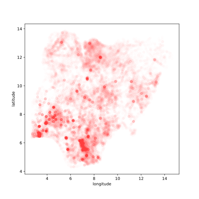

Figure: Location of the over thirty-four thousand health facilities registered in the NMIS data across Nigeria. Each facility plotted according to its latitude and longitude.

Multivariate Regression on Nigeria NMIS Data

Now we will build a design matrix based on the numeric features that include the number of nurses, and the number of midwives, the latitude and longitude. These are our covariates. The response variable will be the number of doctors. We build the design matrix as follows:

Bias as an additional feature.

First we select the covariates and response variables and drop any rows where there are missing values using the pandas dropna method.

covariates = ['num_nurses_fulltime', 'num_nursemidwives_fulltime', 'latitude', 'longitude']
response = ['num_doctors_fulltime']
data_without_missing = data[covariates + response].dropna()

We can see how many rows we have dropped and have a quick sanity check on our new data frame with len.

print(len(data) - len(data_without_missing))

We see that 2,735 of the entries had missing values in one of our variables of interest.

You may also want to use describe or other functions to explore the new data frame.

Now let’s perform a linear regression. But this time, we will create a pandas data frame for the result so we can store it in a form that we can visualize easily.

Phi = data_without_missing[covariates]
Phi['Eins'] = 1 # add a column for the offset
y = data_without_missing[response]

import pandas as pd

w = pd.DataFrame(data=np.linalg.solve(Phi.T@Phi, Phi.T@y),  # solve linear regression here
                 index = Phi.columns,  # columns of Phi become rows of w
                 columns=['regression_coefficient']) # the column of Phi is the value of regression coefficient

We can check the residuals to see how good our estimates are. First we create a pandas data frame containing the predictions and use it to compute the residuals.

ypred = pd.DataFrame(data=(Phi@w).values, columns=['num_doctors_fulltime'])
resid = y-ypred

Let’s look at the residuals. We can use describe to get a summary.

resid.describe()

We can see that while the standard deviation of our residuals is around 3, (this is equivalent to a root mean square error). The smallest and largest residual sow there are some significant outliers that our regression isn’t picking up.

Figure: Residual values for the ratings from the prediction of the movie rating given the data from the film.

Which shows our model hasn’t yet done a great job of representation, because the spread of values is large. We can check what the rating is dominated by in terms of regression coefficients.

w

Checking our regression coefficients, we see that the number of doctors is positively influenced by the number of nurses and the number of midwives. The latitude and longitude have a smaller effect. The bias term (‘eins’) is a small positive offset.

Aside

Just for informational purposes, the actual approach used in software for fitting a linear model should be a QR decomposition.

Solution with QR Decomposition

Performing a solve instead of a matrix inverse is the more numerically stable approach, but we can do even better. A QR-decomposition of a matrix factorizes it into a matrix which is an orthogonal matrix \(\mathbf{Q}\), so that \(\mathbf{Q}^\top \mathbf{Q} = \mathbf{I}\). And a matrix which is upper triangular, \(\mathbf{R}\). \[ \boldsymbol{ \Phi}^\top \boldsymbol{ \Phi}\boldsymbol{\beta} = \boldsymbol{ \Phi}^\top \mathbf{ y} \] and we substitute \(\boldsymbol{ \Phi}= \mathbf{Q}{\mathbf{R}\) so we have \[ (\mathbf{Q}\mathbf{R})^\top (\mathbf{Q}\mathbf{R})\boldsymbol{\beta} = (\mathbf{Q}\mathbf{R})^\top \mathbf{ y} \] \[ \mathbf{R}^\top (\mathbf{Q}^\top \mathbf{Q}) \mathbf{R} \boldsymbol{\beta} = \mathbf{R}^\top \mathbf{Q}^\top \mathbf{ y} \]

\[ \mathbf{R}^\top \mathbf{R} \boldsymbol{\beta} = \mathbf{R}^\top \mathbf{Q}^\top \mathbf{ y} \] \[ \mathbf{R} \boldsymbol{\beta} = \mathbf{Q}^\top \mathbf{ y} \] which leaves us with a lower triangular system to solve.

This is a more numerically stable solution because it removes the need to compute \(\boldsymbol{ \Phi}^\top\boldsymbol{ \Phi}\) as an intermediate. Computing \(\boldsymbol{ \Phi}^\top\boldsymbol{ \Phi}\) is a bad idea because it involves squaring all the elements of \(\boldsymbol{ \Phi}\) and thereby potentially reducing the numerical precision with which we can represent the solution. Operating on \(\boldsymbol{ \Phi}\) directly preserves the numerical precision of the model.

This can be more particularly seen when we begin to work with basis functions in the next session. Some systems that can be resolved with the QR decomposition cannot be resolved by using solve directly.

import scipy as sp

Q, R = np.linalg.qr(Phi)
w = sp.linalg.solve_triangular(R, Q.T@y) 
w = pd.DataFrame(w, index=Phi.columns)
w

Basis Function Models

We are reviewing models that are linear in the parameters. Very often we are interested in non-linear predictions. We can make models that are linear in the parameters and given non-linear predictions by introducing non-linear basis functions. A common example is the polynomial basis.

Polynomial Basis

The polynomial basis combines higher order polynomials together to create the function. For example, the fourth order polynomial has five components to its basis function. \[ \phi_j(x) = x^j \]

import numpy as np

import mlai

from mlai import polynomial

Figure: The set of functions which are combined to form a polynomial basis.

Functions Derived from Polynomial Basis

\[ f(x) = {\color{red}{w_0}} + {\color{magenta}{w_1 x}} + {\color{blue}{w_2 x^2}} + {\color{green}{w_3 x^3}} + {\color{cyan}{w_4 x^4}} \]

Figure: A random combination of functions from the polynomial basis.

The predictions from this model, \[ f(x) = w_0 + w_1 x+ w_2 x^2 + w_3 x^3 + w_4 x^4 \] are linear in the parameters, \(\mathbf{ w}\), but non-linear in the input \(x^3\). Here we are showing a polynomial basis for a 1-dimensional input, \(x\), but basis functions can also be constructed for multidimensional inputs, \(\mathbf{ x}\).}

In the neural network models, the “RELU function” is normally used as a basis function, but for illustration we will continue with the polynomial basis for these linear models.

Olympic Marathon Data

Gold medal times for Olympic Marathon since 1896. Marathons before 1924 didn’t have a standardized distance. Present results using pace per km. In 1904 Marathon was badly organized leading to very slow times.

Image from Wikimedia Commons http://bit.ly/16kMKHQ

The first thing we will do is load a standard data set for regression modelling. The data consists of the pace of Olympic Gold Medal Marathon winners for the Olympics from 1896 to present. Let’s load in the data and plot.

import numpy as np
import pods

data = pods.datasets.olympic_marathon_men()
x = data['X']
y = data['Y']

offset = y.mean()
scale = np.sqrt(y.var())
yhat = (y - offset)/scale

Figure: Olympic marathon pace times since 1896.

Things to notice about the data include the outlier in 1904, in that year the Olympics was in St Louis, USA. Organizational problems and challenges with dust kicked up by the cars following the race meant that participants got lost, and only very few participants completed. More recent years see more consistently quick marathons.

Polynomial Fits to Olympic Marthon Data

import numpy as np

Define the polynomial basis function.

import mlai

from mlai import polynomial

def polynomial(x, num_basis=4, data_limits=[-1., 1.]):
    "Polynomial basis"
    centre = data_limits[0]/2. + data_limits[1]/2.
    span = data_limits[1] - data_limits[0]
    z = np.asarray(x, dtype=float) - centre
    z = 2*z/span   # scale the inputs to be within -1, 1 where polynomials are well behaved
    Phi = np.zeros((x.shape[0], num_basis))
    for i in range(num_basis):
        Phi[:, i:i+1] = z**i
    return Phi

Now we include the solution for the linear regression through QR-decomposition.

def basis_fit(Phi, y):
    "Use QR decomposition to fit the basis."""
    Q, R = np.linalg.qr(Phi)
    return sp.linalg.solve_triangular(R, Q.T@y) 

Linear Fit

poly_args = {'num_basis':2, # two basis functions (1 and x)
             'data_limits':xlim}
Phi = polynomial(x, **poly_args)
w = basis_fit(Phi, y)

Now we make some predictions for the fit.

x_pred = np.linspace(xlim[0], xlim[1], 400)[:, np.newaxis]
Phi_pred = polynomial(x_pred, **poly_args)
f_pred = Phi_pred@w

Figure: Fit of a 1-degree polynomial (a linear model) to the Olympic marathon data.

Cubic Fit

poly_args = {'num_basis':4, # four basis: 1, x, x^2, x^3
             'data_limits':xlim}
Phi = polynomial(x, **poly_args)
w = basis_fit(Phi, y)

Phi_pred = polynomial(x_pred, **poly_args)
f_pred = Phi_pred@w

Figure: Fit of a 3-degree polynomial (a cubic model) to the Olympic marathon data.

9th Degree Polynomial Fit

Now we’ll try a 9th degree polynomial fit to the data.

poly_args = {'num_basis':10, # basis up to x^9
             'data_limits':xlim}
Phi = polynomial(x, **poly_args)
w = basis_fit(Phi, y)

Phi_pred = polynomial(x_pred, **poly_args)
f_pred = Phi_pred@w

Figure: Fit of a 9-degree polynomial to the Olympic marathon data.

16th Degree Polynomial Fit

Now we’ll try a 16th degree polynomial fit to the data.

poly_args = {'num_basis':17, # basis up to x^16
             'data_limits':xlim}
Phi = polynomial(x, **poly_args)
w = basis_fit(Phi, y)

Phi_pred = polynomial(x_pred, **poly_args)
f_pred = Phi_pred@w

Figure: Fit of a 16-degree polynomial to the Olympic marathon data.

26th Degree Polynomial Fit

Now we’ll try a 26th degree polynomial fit to the data.

poly_args = {'num_basis':27, # basis up to x^26
             'data_limits':xlim}
Phi = polynomial(x, **poly_args)
w = basis_fit(Phi, y)

Phi_pred = polynomial(x_pred, **poly_args)
f_pred = Phi_pred@w

Figure: Fit of a 26-degree polynomial to the Olympic marathon data.

The Bootstrap

Bootstrap sampling (Efron, 1979) is an approach to assessing the sensitivity of the model to different variations on a data set. In an ideal world, we’d like to be able to look at different realisations from the original data generating distribution \(\mathbb{P}(y, \mathbf{ x})\), but this is not available to us.

In bootstrap sampling, we take the sample we have, \[ \mathbf{ y}, \mathbf{X}\sim \mathbb{P}(y, \mathbf{ x}) \] and resample from that data, rather than from the true distribution. So, we have a new data set, \(\hat{\mathbf{ y}}\), \(\hat{\mathbf{X}}\) which is sampled from the original with replacement.

import numpy as np

def bootstrap(X):
    "Return a bootstrap sample from a data set."
    n = X.shape[0]
    ind = np.random.choice(n, n, replace=True) # Sample randomly with replacement.
    return X[ind, :]  

Bootstrap and Olympic Marathon Data

First we define a function to bootstrap resample our dataset.

import numpy as np

def bootstrap(X, y):
    "Return a bootstrap sample from a data set."
    n = X.shape[0]
    ind = np.random.choice(n, n, replace=True) # Sample randomly with replacement.
    return X[ind, :], y[ind, :]

num_bootstraps = 10

def bootstrap_fit(Phi, y, size):
    W = np.zeros((Phi.shape[1], size))
    for i in range(size):
        Phi_hat, y_hat = bootstrap(Phi, y)
        W[:, i:i+1] = basis_fit(Phi_hat, y_hat)
    return W

Linear Fit

poly_args = {'num_basis':2, # two basis functions (1 and x)
             'data_limits':xlim}
Phi = polynomial(x, **poly_args)
W_hat = bootstrap_fit(Phi, y, num_bootstraps)

Now we make some predictions for the fit.

x_pred = np.linspace(xlim[0], xlim[1], 400)[:, np.newaxis]
Phi_pred = polynomial(x_pred, **poly_args)
f_pred = Phi_pred@W_hat

Figure: Fit of a 1 degree polynomial (a linear model) to the olympic marathon data.

Cubic Fit

poly_args = {'num_basis':4, # four basis: 1, x, x^2, x^3
             'data_limits':xlim}
Phi = polynomial(x, **poly_args)
W_hat = bootstrap_fit(Phi, y, num_bootstraps)

Phi_pred = polynomial(x_pred, **poly_args)
f_pred = Phi_pred@W_hat

Figure: Fit of a 3 degree polynomial (a cubic model) to the olympic marathon data.

9th Degree Polynomial Fit

Now we’ll try a 9th degree polynomial fit to the data.

poly_args = {'num_basis':10, # basis up to x^9
             'data_limits':xlim}
Phi = polynomial(x, **poly_args)
W_hat = bootstrap_fit(Phi, y, num_bootstraps)

Phi_pred = polynomial(x_pred, **poly_args)
f_pred = Phi_pred@W_hat

Figure: Fit of a 9 degree polynomial to the olympic marathon data.

16th Degree Polynomial Fit

Now we’ll try a 16th degree polynomial fit to the data.

poly_args = {'num_basis':17, # basis up to x^16
             'data_limits':xlim}
Phi = polynomial(x, **poly_args)
W_hat = bootstrap_fit(Phi, y, num_bootstraps)

Phi_pred = polynomial(x_pred, **poly_args)
f_pred = Phi_pred@W_hat

Figure: Fit of a 16 degree polynomial to the olympic marathon data.

Bias Variance Decomposition

One of Breiman’s ideas for improving predictive performance is known as bagging (Breiman:bagging96?). The idea is to train a number of models on the data such that they overfit (high variance). Then average the predictions of these models. The models are trained on different bootstrap samples (Efron, 1979) and their predictions are aggregated giving us the acronym, Bagging. By combining decision trees with bagging, we recover random forests (Breiman, 2001).

Bias and variance can also be estimated through Efron’s bootstrap (Efron, 1979), and the traditional view has been that there’s a form of Goldilocks effect, where the best predictions are given by the model that is ‘just right’ for the amount of data available. Not to simple, not too complex. The idea is that bias decreases with increasing model complexity and variance increases with increasing model complexity. Typically plots begin with the Mummy bear on the left (too much bias) end with the Daddy bear on the right (too much variance) and show a dip in the middle where the Baby bear (just) right finds themselves.

The Daddy bear is typically positioned at the point where the model can exactly interpolate the data. For a generalized linear model (McCullagh and Nelder, 1989), this is the point at which the number of parameters is equal to the number of data¹.

The bias-variance decomposition (Geman:biasvariance92?) considers the expected test error for different variations of the training data sampled from, \(\mathbb{P}(\mathbf{ x}, y)\) \[\begin{align*} R(\mathbf{ w}) = & \int \left(y- f^*(\mathbf{ x})\right)^2 \mathbb{P}(y, \mathbf{ x}) \text{d}y\text{d}\mathbf{ x}\\ & \triangleq \mathbb{E}\left[ \left(y- f^*(\mathbf{ x})\right)^2 \right]. \end{align*}\]

This can be decomposed into two parts, \[ \begin{align*} \mathbb{E}\left[ \left(y- f(\mathbf{ x})\right)^2 \right] = & \text{bias}\left[f^*(\mathbf{ x})\right]^2 + \text{variance}\left[f^*(\mathbf{ x})\right] +\sigma^2, \end{align*} \] where the bias is given by \[ \text{bias}\left[f^*(\mathbf{ x})\right] = \mathbb{E}\left[f^*(\mathbf{ x})\right] - f(\mathbf{ x}) \] and it summarizes error that arises from the model’s inability to represent the underlying complexity of the data. For example, if we were to model the marathon pace of the winning runner from the Olympics by computing the average pace across time, then that model would exhibit bias error because the reality of Olympic marathon pace is it is changing (typically getting faster).

The variance term is given by \[ \text{variance}\left[f^*(\mathbf{ x})\right] = \mathbb{E}\left[\left(f^*(\mathbf{ x}) - \mathbb{E}\left[f^*(\mathbf{ x})\right]\right)^2\right]. \] The variance term is often described as arising from a model that is too complex, but we must be careful with this idea. Is the model really too complex relative to the real world that generates the data? The real world is a complex place, and it is rare that we are constructing mathematical models that are more complex than the world around us. Rather, the ‘too complex’ refers to ability to estimate the parameters of the model given the data we have. Slight variations in the training set cause changes in prediction.

Models that exhibit high variance are sometimes said to ‘overfit’ the data whereas models that exhibit high bias are sometimes described as ‘underfitting’ the data.

Also related on generalization error is the so called ‘no free lunch theorem’, which refers to our inability to decide what a better learning algorithm is without making assumptions about the data (Wolpert, 1996) (see also Wolpert (2002)).

Regularization

The solution to the linear system is given by solving, \[ \boldsymbol{ \Phi}^\top\boldsymbol{ \Phi}\mathbf{ w}= \boldsymbol{ \Phi}^\top\mathbf{ y} \] for \(\mathbf{ w}\).

But if \(\boldsymbol{ \Phi}^\top\boldsymbol{ \Phi}\) is not full rank, this system cannot be solved. This is reflective of an underdetermined system of equations. There are infinite solutions. This happens when there are more basis functions than data points, in effect the number of data we have is not enough to determine the parameters.

Thinking about this in terms of the Hessian, if \(\boldsymbol{ \Phi}^\top\boldsymbol{ \Phi}\) is not full rank, then we are no longer at a minimum. We are in a trough, because not full rank implies that there are fewer eigenvectors than dimensions, in effect for those dimensions where there is no eigenvector, the objective function is ‘flat’. It is ambivalent to changes in parameters. This implies there are infinite valid solutions.

One solution to this problem is to regularize the system.

Coefficient Shrinkage

Coefficient shrinkage is a technique where the parameters of the of the model are ‘encouraged’ to be small. In practice this is normally done by augmenting the objective function with a term that keeps the parameters low, typically by penalizing a norm.

Tikhonov Regularization

In neural network models this approach is sometimes called ‘weight decay’. At every gradient step we reduce the value of the weight a little. This idea comes from an approach called Tikhonov regularization (Tikhonov and Arsenin, 1977), where the objective function is augmented by the L2 norm of the weights, \[ L(\mathbf{ w}) = (\mathbf{ y}- \mathbf{ f})^\top(\mathbf{ y}- \mathbf{ f}) + \alpha\left\Vert \mathbf{W} \right\Vert_2^2 \] with some weighting \(\alpha >0\). This has the effect of changing the Hessian at the minimum to \[ \boldsymbol{ \Phi}^\top\boldsymbol{ \Phi}+ \alpha \mathbf{I} \] Which is always full rank. The minimal eigenvalues are now given by \(\alpha\).

Lasso

Other techniques for regularization based on a norm of the parameters include the Lasso (Tibshirani, 1996), which is an L1 norm of the parameters

Splines, Functions, Hilbert Kernels

Regularization of the parameters has the desired effect of making the solution viable, but it can sometimes be difficult to interpret, particularly if the parameters don’t have any inherent meaning (like in a neural network). An alternative approach is to regularize the function, \(\mathbf{ f}\), directly, (see e.g., Kimeldorf and Wahba (1970) and Wahba (1990)). This is the approach taken by spline models which use energy-based regularization for \(f(\cdot)\) and also kernel methods such as the support vector machine (Schölkopf and Smola, 2001).

Training with Noise

In practice, and across the last two waves of neural networks, other techniques for regularization have been used which can be seen as perturbing the neural network in some way. For example, in dropout (Srivastava et al., 2014), different basis functions are eliminated from the gradient computation at each gradient update.

Many of these perturbations have some form of regularizing effect. The exact nature of the effect is not always easy to characterize, but in some cases, we can assess how these manipulations effect the model. For example, Bishop (1995) analyzed training with ‘noisy inputs’ and showed conditions under which it’s equivalent to Tikhonov regularization.

But in general, these approaches can have different interpretations and they’ve also been related to ensemble learning (e.g. related to bagging or Bayesian approaches).

Shallow and Deep Learning

So far, we have been talking about linear models or shallow learning as we might think of it. Let’s pause for a moment and consider a fully connected deep neural network model to relate the two ideas.

Deep Neural Network

%pip install daft

Figure: A deep neural network. Input nodes are shown at the bottom. Each hidden layer is the result of applying an affine transformation to the previous layer and placing through an activation function.

Mathematically, each layer of a neural network is given through computing the activation function, \(\phi(\cdot)\), contingent on the previous layer, or the inputs. In this way the activation functions, are composed to generate more complex interactions than would be possible with any single layer. \[ \begin{align*} \mathbf{ h}_{1} &= \phi\left(\mathbf{W}_1 \mathbf{ x}\right)\\ \mathbf{ h}_{2} &= \phi\left(\mathbf{W}_2\mathbf{ h}_{1}\right)\\ \mathbf{ h}_{3} &= \phi\left(\mathbf{W}_3 \mathbf{ h}_{2}\right)\\ f&= \mathbf{ w}_4 ^\top\mathbf{ h}_{3} \end{align*} \]

Under our basis function perspective, we can see that our deep neural network is mathematical composition of basis function models. Each layer contains a separate basis function set, so \[ f(\mathbf{ x}; \mathbf{W}) = \mathbf{ w}_4 ^\top\phi\left(\mathbf{W}_3 \phi\left(\mathbf{W}_2\phi\left(\mathbf{W}_1 \mathbf{ x}\right)\right)\right). \]

In this course there are two reasons for looking at the shallow model. Firstly, it is easier to introduce the concepts of regularisation in the linear model regime. Secondly, the matrix forms we see, e.g., expressions like \(\boldsymbol{ \Phi}^\top \boldsymbol{ \Phi}\), appear in both models.

For deep learning, we can no longer optimize the parameters of the model through solving a linear system². Instead, we need to turn to non-linear optimization algorithms. For deep learning, that’s typically stochastic gradient descent.

While it’s possible to compute the Hessian in a neural network, Bishop (1992), we also find that it varies across the parameter space and will not normally be positive definite. In practice, the number of parameters is normally so large that storing the Hessian is impossible (it has quadratic cost in the number of weights/parameters) due to memory constraints.

This means that while the theory of minima in optimization is well understood, empirical experiments with large neural networks are hard and the lessons of small models do not all translate to the very large systems.

We can stay within the framework of linear models but take a step closer to neural network models by introducing functions that are non-linear in the inputs, \(\mathbf{ x}\), known as basis functions.

Overparameterised Systems

If we could examine the Hessian of a neural network at its minimum, we can speculate about what we would find. In particular, we would find that it would have very many low (or negative) eigenvalues in many directions. This is indicative of the parameters being badly determined because of the neural network model being heavily overparameterized. So how does it generalize?

Simply put, there is not enough regularization encoded in the objective function of the neural network models we are using to explain the generalization performance. There must be something in the algorithms we are using that causes these highly overparameterized models to generalise well.

Double Descent

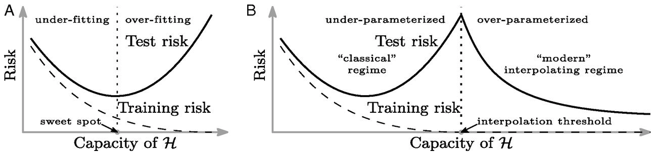
Figure: Left traditional perspective on generalization. There is a sweet spot of operation where the training error is still non-zero. Overfitting occurs when the variance increases. Right The double descent phenomenon, the modern models operate in an interpolation regime where they reconstruct the training data fully but are well regularized in their interpolations for test data. Figure from Belkin et al. (2019).

But the modern empirical finding is that when we move beyond Daddy bear, into the dark forest of the massively overparameterized model we can achieve good generalization. Indeed, recent work is showing that large language models are even memorizing data (Carlini et al., 2020) like non-parametric models do.

As Zhang et al. (2017) starkly illustrated with their random labels experiment, within the dark forest there are some terrible places, big bad wolves of overfitting that will gobble up your model. But as empirical evidence shows there is also a safe and hospitable Grandma’s house where these highly overparameterized models are safely consumed. Fundamentally, it must be about the route you take through the forest, and the precautions you take to ensure the wolf doesn’t see where you’re going and beat you to the door.

There are two implications of this empirical result. Firstly, that there is a great deal of new theory that needs to be developed. Secondly, that theory is now obliged to conflate two aspects to modelling that we generally like to keep separate: the model and the algorithm.

Classical statistical theory around predictive generalization focusses specifically on the class of models that is being used for data fitting. Historically, whether that theory follows a Fisher-aligned estimation approach (see e.g., Vapnik (1998)) or model-based Bayesian approach (see e.g., Ghahramani (2015)), neither is fully equipped to deal with these new circumstances because, to continue our rather tortured analogy, these theories provide us with a characterization of the destination of the algorithm, and seek to ensure that we reach that destination. Modern machine learning requires theories of the journey and what our route through the forest should be.

Crucially, the destination is always associated with 100% accuracy on the training set. An objective that is always achievable for the overparameterized model.

Intuitively, it seems that a highly overparameterized model places Grandma’s house on the edge of the dark forest. Making it easily and quickly accessible to the algorithm. The larger the model, the more exposed Grandma’s house becomes. Perhaps this is due to some form of blessing of dimensionality brings Grandma’s house closer to the edge of the forest in a high dimensional setting. Really, we should think of Grandma’s house as a low dimensional manifold of destinations that are safe. A path through the forest where the wolf of overfitting doesn’t venture. In the GLM case, we know already that when the number of parameters matches the number of data there is precisely one location in parameter space where accuracy on the training data is 100%. Our previous misunderstanding of generalization stemmed from the fact that (seemingly) it is highly unlikely that this single point is a good place to be from the perspective of generalization. Additionally, it is often difficult to find. Finding the precise polynomial coefficients in a least squares regression to exactly fit the basis to a small data set such as the Olympic marathon data requires careful consideration of the numerical properties and an orthogonalization of the design matrix (Lawson and Hanson, 1995).

It seems that with a highly overparameterized model, these locations become easier to find and they provide good generalization properties. In machine learning this is known as the “double descent phenomenon” (see e.g., Belkin et al. (2019)).

See also this talk by Misha Belkin: http://www.ipam.ucla.edu/abstract/?tid=15552&pcode=GLWS4 and these related papers https://www.pnas.org/content/116/32/15849.short, https://www.pnas.org/content/117/20/10625

Neural Tangent Kernel

Another approach to analysis exploits the fact that optimization is occurring in a very high dimensional parameter space. By considering initializations that involve small random weights (known as the NTK initialization) and noting that small updates in the learning mean that the model doesn’t move far from this initialization (Jacot et al., 2018).

For very wide neural networks, when these conditions are fulfilled, the network can be approximately represented by a kernel known as the neural tangent kernel. A kernel is a regularizer that operates in function space rather than feature space.

Regularization in Optimization

Another interesting theoretical direction is to study the path that neural network algorithms take when finding the optima. For certain simple linear systems, you can analytically study the ‘gradient flow’.

Neural networks are normally trained by (stochastic) gradient descent. This is a discrete optimization algorithm where at each point, a step in the direction of the (approximate) gradient is taken.

Gradient flow replaces this discrete update with a differential equation, where the step at any point is an exact gradient update. As a result, the path of the optimization can be studied as a differential equation.

By making assumptions about the initialization, the optimum that gradient flow will find can be characterised. For a highly overparameterized linear model, Gunasekar et al. (2017) show in matrix factorization, that for particular initializations, the optimum will be a global optimum of the objective that minimizes the L2-norm.

By reparameterizing the linear model so that each \(w_i = u_i^2 - v_i^2\) and optimising in the space defined by \(\mathbf{u}\) and \(\mathbf{v}\) Woodworth et al. (2020) show that the L1 norm is found.

Other papers have looked at deep linear models (Arora et al., 2019) where \[ f(\mathbf{ x}; \mathbf{W}) = \mathbf{W}_4 \mathbf{W}_3 \mathbf{W}_2 \mathbf{W}_1 \mathbf{ x}. \] In these models, a gradient flow analysis shows that the model finds solutions where the linear mapping, \[ \mathbf{W}= \mathbf{W}_4 \mathbf{W}_3 \mathbf{W}_2 \mathbf{W}_1 \] is very low rank. This is highly suggestive of another type of regularization that could be occurring in deep neural networks. Low rank parameter matrices mean that the effective capacity of the neural network is reduced. Indeed, empirical observations of the rank of deep nets trained on data suggest that they may be finding such solutions.

Thanks!

For more information on these subjects and more you might want to check the following resources.

• twitter: @lawrennd
• podcast: The Talking Machines
• newspaper: Guardian Profile Page
• blog: http://inverseprobability.com

References

bootstrap

David Hogg’s lecture https://speakerdeck.com/dwhgg/linear-regression-with-huge-numbers-of-parameters

The Deep Bootstrap https://twitter.com/PreetumNakkiran/status/1318007088321335297?s=20

Aki Vehtari on Leave One Out Uncertainty: https://arxiv.org/abs/2008.10296 (check for his references).