Generalization and Neural Networks

Quadratic Loss and Linear System

Expected Loss

\[ R(\mathbf{ w}) = \int L(y, x, \mathbf{ w}) \mathbb{P}(y, x) \text{d}y \text{d}x. \]

Sample-Based Approximations

• Sample based approximation: replace true expectation with sum over samples. \[ \int f(z) p(z) \text{d}z\approx \frac{1}{s}\sum_{i=1}^s f(z_i). \]

• Allows us to approximate true integral with a sum \[ R(\mathbf{ w}) \approx \frac{1}{n}\sum_{i=1}^{n} L(y_i, x_i, \mathbf{ w}). \]

Basis Function Models

Polynomial Basis

\[ \phi_j(x) = x^j \]

❮ ❯

Functions Derived from Polynomial Basis

\[ f(x) = {\color{cyan}{w_0}} + {\color{green}{w_1 x}} + {\color{yellow}{w_2 x^2}} + {\color{magenta}{w_3 x^3}} + {\color{red}{w_4 x^4}} \]

❮ ❯

• _2 ^2 + _3 ^3 + _4 ^4 $$ are linear in the parameters, \(\mathbf{ w}\), but non-linear in the input \(x^3\). Here we are showing a polynomial basis for a 1-dimensional input, \(x\), but basis functions can also be constructed for multidimensional inputs, \(\mathbf{ x}\).}

Olympic Marathon Data

Gold medal times for Olympic Marathon since 1896. Marathons before 1924 didn’t have a standardized distance. Present results using pace per km. In 1904 Marathon was badly organized leading to very slow times.

Image from Wikimedia Commons http://bit.ly/16kMKHQ

Olympic Marathon Data

Polynomial Fits to Olympic Marthon Data

• Fit linear model with polynomial basis to marathon data.
• Try different numbers of basis functions (different degress of polynomial).
• Check the quality of fit.

Linear Fit

\[f(x, \mathbf{ w}) = w_0 + w_1x\]

Cubic Fit

\[f(x, \mathbf{ w}) = w_0 + w_1 x+ w_2 x^2 + w_3 x^3\]

9th Degree Polynomial Fit

\[f(x, \mathbf{ w}) = w_0 + w_1 x+ w_2 x^2 + \dots + w_9 x^9\]

16th Degree Polynomial Fit

\[f(x, \mathbf{ w}) = w_0 + w_1 x+ w_2 x^2 + \dots + w_{16} x^{16}\]

26th Degree Polynomial Fit

\[f(x, \mathbf{ w}) = w_0 + w_1 x+ w_2 x^2 + \dots + w_{26} x^{26}\]

The Bootstrap

\[ \mathbf{ y}, \mathbf{X}\sim \mathbb{P}(y, \mathbf{ x}) \]

Resample Dataset

def bootstrap(X):
    "Return a bootstrap sample from a data set."
    n = X.shape[0]
    ind = np.random.choice(n, n, replace=True) # Sample randomly with replacement.
    return X[ind, :]

Bootstrap and Olympic Marathon Data

Linear Fit

\[f(x, \mathbf{ w}) = w_0 + w_1 x\]

Cubic Fit

\[f(x, \mathbf{ w}) = w_0 + w_1 x+ w_2 x^2 + w_{3} x^3\]

9th Degree Polynomial Fit

\[f(x, \mathbf{ w}) = w_0 + w_1 x+ w_2 x^2 + \dots + w_{9} x^{9}\]

16th Degree Polynomial Fit

\[f(x, \mathbf{ w}) = w_0 + w_1 x+ w_2 x^2 + \dots + w_{16} x^{16}\]

Bias Variance Decomposition

Generalisation error \[\begin{align*} R(\mathbf{ w}) = & \int \left(y- f^*(\mathbf{ x})\right)^2 \mathbb{P}(y, \mathbf{ x}) \text{d}y\text{d}\mathbf{ x}\\ & \triangleq \mathbb{E}\left[ \left(y- f^*(\mathbf{ x})\right)^2 \right]. \end{align*}\]

Decompose

Decompose as \[ \begin{align*} \mathbb{E}\left[ \left(y- f(\mathbf{ x})\right)^2 \right] = & \text{bias}\left[f^*(\mathbf{ x})\right]^2 \\ & + \text{variance}\left[f^*(\mathbf{ x})\right] \\ \\ &+\sigma^2, \end{align*} \]

Bias

• Given by \[ \text{bias}\left[f^*(\mathbf{ x})\right] = \mathbb{E}\left[f^*(\mathbf{ x})\right] - f(\mathbf{ x}) \]

• Error due to bias comes from a model that’s too simple.

Variance

• Given by \[ \text{variance}\left[f^*(\mathbf{ x})\right] = \mathbb{E}\left[\left(f^*(\mathbf{ x}) - \mathbb{E}\left[f^*(\mathbf{ x})\right]\right)^2\right]. \]

• Slight variations in the training set cause changes in the prediction. Error due to variance is error in the model due to an overly complex model.

Regularization

Linear system, solve:

\[ \boldsymbol{ \Phi}^\top\boldsymbol{ \Phi}\mathbf{ w}= \boldsymbol{ \Phi}^\top\mathbf{ y} \] But if \(\boldsymbol{ \Phi}^\top\boldsymbol{ \Phi}\) then this is not well posed.

Tikhonov Regularization

• Updated objective: \[ L(\mathbf{ w}) = (\mathbf{ y}- \mathbf{ f})^\top(\mathbf{ y}- \mathbf{ f}) + \alpha\left\Vert \mathbf{W} \right\Vert_2^2 \]
• Hessian: \[ \boldsymbol{ \Phi}^\top\boldsymbol{ \Phi}+ \alpha \mathbf{I} \]

Splines, Functions, Hilbert Kernels

• Can also regularize the function \(f(\cdot)\) directly.
• This approach taken in splines and Wahba (1990) and kernels Schölkopf and Smola (2001).
• Mathematically more elegant, but algorithmically less flexible and harder to scale.

Training with Noise

• Other regularisation approaches such as dropout (Srivastava et al., 2014)
• Often perturbing the neural network structure or inputs.
• Can have elegant interpretations (see e.g. Bishop (1995))
• Also interpreted as ensemble or Bayesian methods.

Shallow and Deep Learning

Deep Neural Network

Deep Neural Network

Mathematically

\[ \begin{align*} \mathbf{ h}_{1} &= \phi\left(\mathbf{W}_1 \mathbf{ x}\right)\\ \mathbf{ h}_{2} &= \phi\left(\mathbf{W}_2\mathbf{ h}_{1}\right)\\ \mathbf{ h}_{3} &= \phi\left(\mathbf{W}_3 \mathbf{ h}_{2}\right)\\ f&= \mathbf{ w}_4 ^\top\mathbf{ h}_{3} \end{align*} \]

Neural Network Prediction Function

\[ f(\mathbf{ x}; \mathbf{W}) = \mathbf{ w}_4 ^\top\phi\left(\mathbf{W}_3 \phi\left(\mathbf{W}_2\phi\left(\mathbf{W}_1 \mathbf{ x}\right)\right)\right). \]

Overparameterised Systems

• Neural networks are highly overparameterised.
• If we could examine their Hessian at “optimum”
  • Very low (or negative) eigenvalues.
  • Error function is not sensitive to changes in parameters.
  • Implies parmeters are badly determined

Whence Generalisation?

• Not enough regularisation in our objective functions to explain.
• Neural network models are not using traditional generalisation approaches.
• The ability of these models to generalise must be coming somehow from the algorithm*
• How to explain it and control it is perhaps the most interesting theoretical question for neural networks.

Double Descent

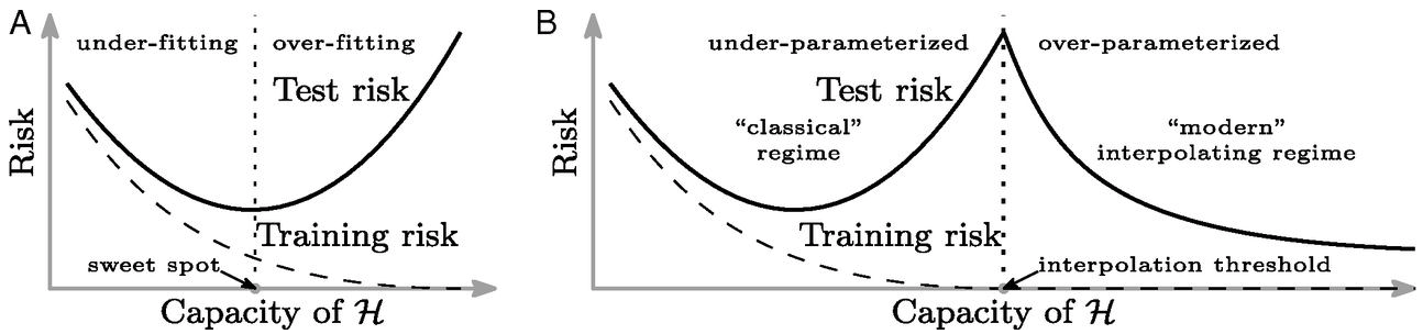
Neural Tangent Kernel

• Consider very wide neural networks.
• Consider particular initialisation.
• Deep neural network is regularising with a particular kernel.
• This is known as the neural tangent kernel (Jacot et al., 2018).

Regularization in Optimization

• Gradient flow methods allow us to study nature of optima.
• In particular systems, with given initialisations, we can show L1 and L2 norms are minimised.
• In other cases the rank of \(\mathbf{W}\) is minimised.
• Questions remain over the nature of this regularisation in neural networks.

Deep Linear Models

\[ f(\mathbf{ x}; \mathbf{W}) = \mathbf{W}_4 \mathbf{W}_3 \mathbf{W}_2 \mathbf{W}_1 \mathbf{ x}. \]

\[ \mathbf{W}= \mathbf{W}_4 \mathbf{W}_3 \mathbf{W}_2 \mathbf{W}_1 \]