Week 1: Introduction

[Powerpoint][jupyter][google colab][reveal]

Neil D. Lawrence

Abstract:

This lecture will give the background to what this course is about, and how it fits in to other material you can find on deep neural network models. It explains deep neural networks are, how they fit into the wider context of the field and why they are successful.

Course Overview

Deep Neural Networks is an eight we course that introduces you to the fundamental concepts behind deep learning with neural networks. Over the last decade, deep neural network models have been behind some of the most impressive feats in machine learning. From the convolutional neural networks that made breakthrough progress on the ImageNet challenge, object detection and the image net challenge, and most recently with the CASP14 Protein Folding result from DeepMind.

Welcome to this course, which is designed to introduce you to the principles and ideas behind deep neural network models.

Due to widespread international interest in neural networks, there is now a great deal of material to help you train and deploy these models. It is not our aim to substitute this material but to augment it with deeper understanding of the reasons why deep learning is successful and the context in which that success has occurred.

You are strongly encouraged to explore that material. For example, you can find Yann LeCun’s neural networks course from NYU here. For example, here is their introductory session with Yann giving the first lecture available here.

Figure: Lecture from the NYU course on Deep Learning given by Yann LeCun, Alfredo Canziani and Mark Goldstein

The full playlist is available here.

Our course is taught by Ferenc Huszár, Nic Lane and Neil Lawrence.

Alongside such teaching material there are frameworks such as PyTorch, that help you in constructing these models and deploying the training on GPUs.

Neural network models are not new, and this is not the first wave of interest in them, it is the third wave. There are reasons why they have become more successful in this wave than in their first two incarnations. Those reasons include the context in which they were reintroduced. In particular, the wide availability of data and fast compute have been critical in their success.

Our aim is to give you the understanding of that context, and therefore deepen your understanding of neural networks, how and when they should be used. The neural network is not a panacea, it does not solve all the challenges of machine learning (at least not in its current incarnation). But it is a powerful framework for flexible modelling of data. Just like any powerful framework, it is important to understand its strengths as well as its limitations.

Schedule

• Week 1:
  1. Introduction and Data. Lecturer: Neil D. Lawrence
  2. Generalisation and Neural Networks. Lecturer: Neil D. Lawrence
• Week 2:
  1. Automatic Differentiation. Lecturer: Ferenc Huszár
  2. Optimization and Stochastic Gradient Descent. Lecturer: Ferenc Huszár
• Week 3:
  1. Hardware. Lecturer: Nic Lane
  2. Summary and Gap Filling: Ferenc Huszár, Neil D. Lawrence, Nic Lane

Set Assignment 1 (30%)

• Week 4:
  1. Convolutional Neural Networks: Nic Lane
  2. Recurrent Neural Networks: Ferenc Huszár

Assignment 1 Submitted

• Week 5:
  1. Sequence to Sequence and Attention: Ferenc Huszár
  2. Transformers: Nic Lane

Set Assignment 2 (70%)

Special Topics

Weeks 6-8 will involve a series of guest lectures and discussion sessions to relate the fundamental material you’ve learnt about to how people are deploying these models in the real world and how they are innovating with these models to extend their capabilities.

The two assignments will make up the entire mark of the module. They should be submitted via Moodle.

What is Machine Learning?

What is machine learning? At its most basic level machine learning is a combination of

\[\text{data} + \text{model} \stackrel{\text{compute}}{\rightarrow} \text{prediction}\]

where data is our observations. They can be actively or passively acquired (meta-data). The model contains our assumptions, based on previous experience. That experience can be other data, it can come from transfer learning, or it can merely be our beliefs about the regularities of the universe. In humans our models include our inductive biases. The prediction is an action to be taken or a categorization or a quality score. The reason that machine learning has become a mainstay of artificial intelligence is the importance of predictions in artificial intelligence. The data and the model are combined through computation.

In practice we normally perform machine learning using two functions. To combine data with a model we typically make use of:

a prediction function it is used to make the predictions. It includes our beliefs about the regularities of the universe, our assumptions about how the world works, e.g., smoothness, spatial similarities, temporal similarities.

an objective function it defines the ‘cost’ of misprediction. Typically, it includes knowledge about the world’s generating processes (probabilistic objectives) or the costs we pay for mispredictions (empirical risk minimization).

The combination of data and model through the prediction function and the objective function leads to a learning algorithm. The class of prediction functions and objective functions we can make use of is restricted by the algorithms they lead to. If the prediction function or the objective function are too complex, then it can be difficult to find an appropriate learning algorithm. Much of the academic field of machine learning is the quest for new learning algorithms that allow us to bring different types of models and data together.

A useful reference for state of the art in machine learning is the UK Royal Society Report, Machine Learning: Power and Promise of Computers that Learn by Example.

You can also check my post blog post on What is Machine Learning?.

Ingredients

The three key ingredients of machine learning are a model, data and compute. Note, that this necessarily implies that an algorithm exists to combine the model with the data and that algorithm is what consumes the compute.

So how do these ingredients pan out in our recipe for deep learning? To better understand this, we’re going to add more historical context and go back go 1997 when, here in Cambridge, there was a six-month programme at the Isaac Newton Institute run on Machine Learning, Neural Networks and Generalisation.

Cybernetics, Neural Networks and the Ratio Club

This is certainly not the first wave of excitement in neural networks. This history of neural networks predates the history of the computer, and papers on neural networks predate papers on the digital computer.

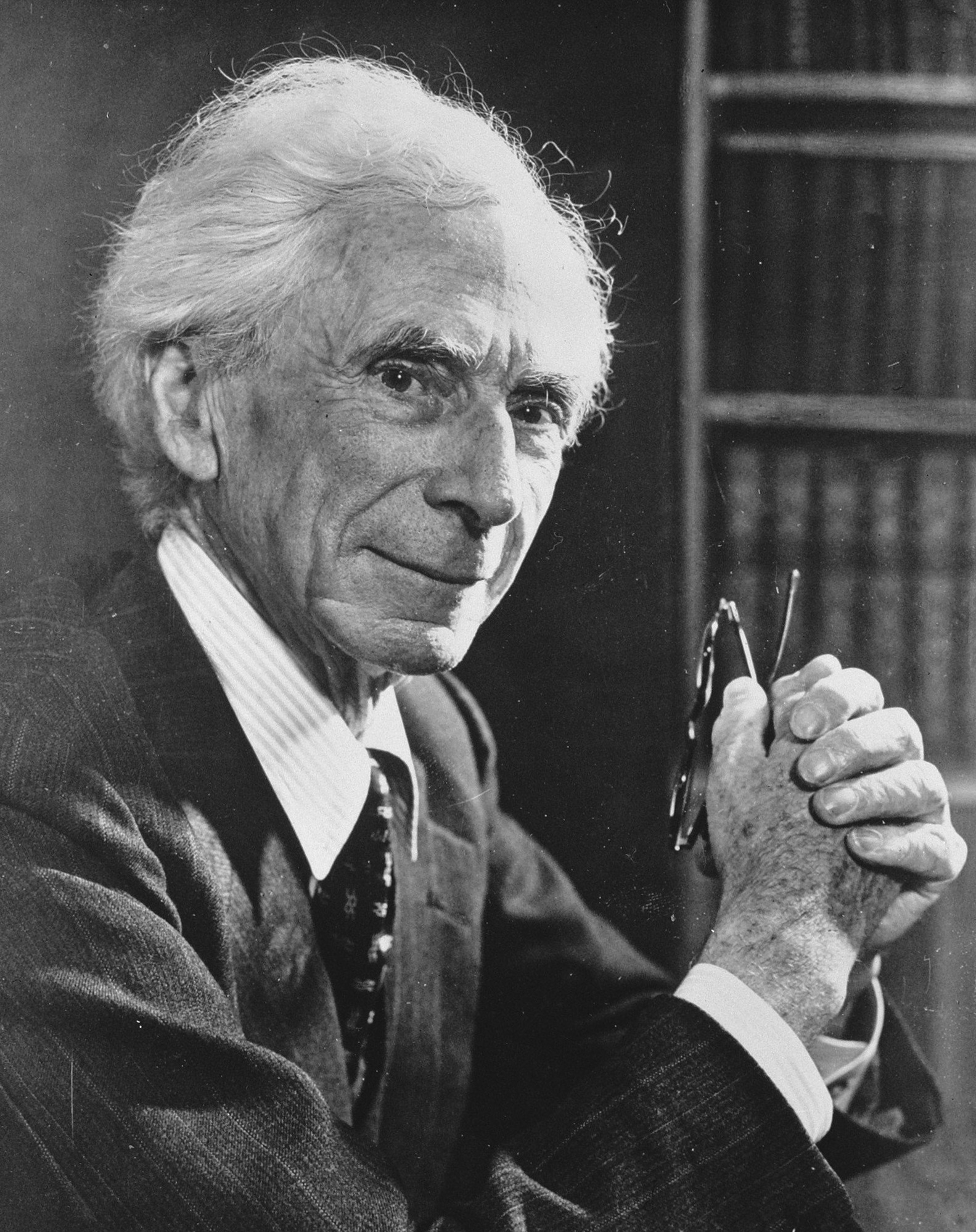
Figure: Bertrand Russell (1872-1970), Walter Pitts, right (1923-1969), Warren McCulloch (1898-1969)

Specifically, one of the first papers on neural networks was written by two collaborators from logic and psychology in 1943. Walter Pitts was a child prodigy who read Russell and Whitehead’s Principia Mathematica. He felt he’d spotted some errors in the text and wrote to Russell in Cambridge, who replied inviting him for a visit. Pitts did not take up the offer because he was only 12 years old. But, three years later, when Russell took a sabbatical at the University of Chicago, Pitts left his home in Detroit and headed to Chicago to hear Russell speak. When Russell left Pitts stayed on studying logic. He never formally took a degree but just worked with whoever was available.

Warren McCulloch was a psychologist who moved to the University of Chicago in 1941. Overlapping interests meant that he met Pitts, who was still living an itinerant lifestyle around the campus of the University. McCulloch invited Pitts to live with his family and they began collaborating on a simple model of the neuron and how neurons might interact. The dominant ‘theory of knowledge’ at the time was logic and their paper attempted to show how networks of neurons. Their paper, A Logical Calculus of the Ideas Immanent in Nervous Activity (McCulloch and Pitts, 1943), was published in the middle of the Second World War. It modelled the neuron as a linear threshold and described how networks of such neurons could create logical functions. The inspiration in the paper is clear, they make use of Rudolf Carnap’s Language II (Carnap, 1937) to represent their theorem and cite the second edition of Russell and Whitehead (Russell and Whitehead, 1925).

Cybernetics

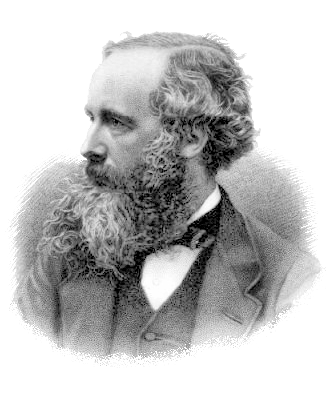
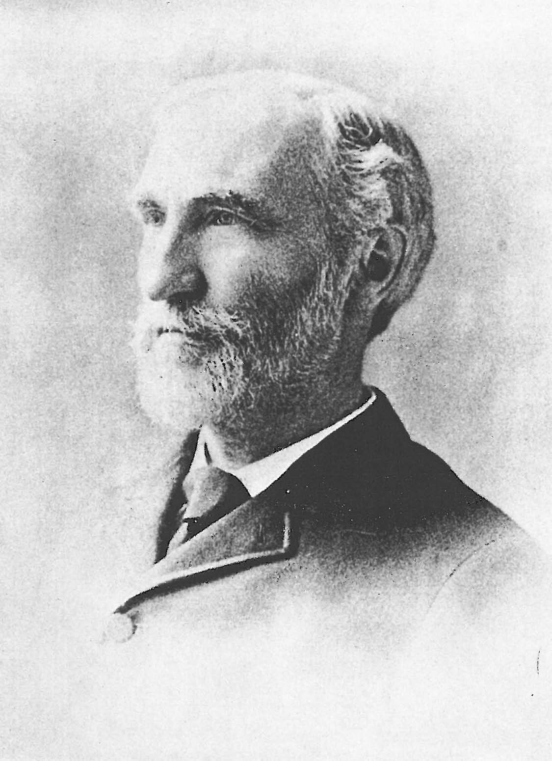
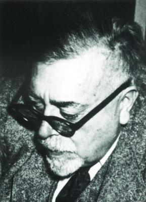
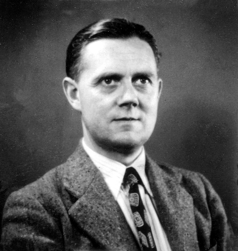
Figure: James Clerk Maxwell (1831-1879), Josiah Willard Gibbs (1839-1903), Norbert Wiener (1894-1964)

After the war, this work, along with McCulloch and Pitts, was at the heart of a movement known as Cybernetics. A term coined by Norbert Wiener (Wiener, 1948) to reflect the wealth of work on sensing and computing. Wiener chose the term as an alternative rendering of the word governor. Governor comes to us from Latin but is a corruption of the Greek κυβερνήτης meaning helmsman. Wiener’s choice of the term was a nod to the importance of James Clerk Maxwell’s work on understanding surging in James Watt’s steam engine governor (Maxwell, 1867). It reflected the importance that Wiener placed on feedback in these systems. From this strand of work came the field of control theory.

Many of the constituent ideas of Cybernetics came from the war itself. Norbert Wiener was a Professor of Applied Mathematics at MIT. He was another child prodigy who visited Russell in Cambridge having completed his PhD at Harvard by the age of 19. But Wiener was less keen on logic than McCulloch and Pitts, he looked to stochastic processes and probability theory as the key to intelligent decision making. He rejected the need for a ‘theory of knowledge’ and preferred to think of a ‘theory of ignorance’ which was inspired by statistical mechanics, Maxwell was also an originator of the field, but Wiener wrote of Josiah Willard Gibbs as being his inspiration.

This nascent community was mainly based on those who were involved in war work. Wiener worked on radar systems for tracking aircraft (leading to the Wiener filter (Wiener, 1949)). In the UK researchers such as Jack Good, Alan Turing, Donald MacKay, Ross Ashby formed the Ratio Club. A group of scientists interested in how the brain works and how it might be modelled. Many of these scientists also worked on radar systems or code breaking.

Analogue and Digital

Donald MacKay

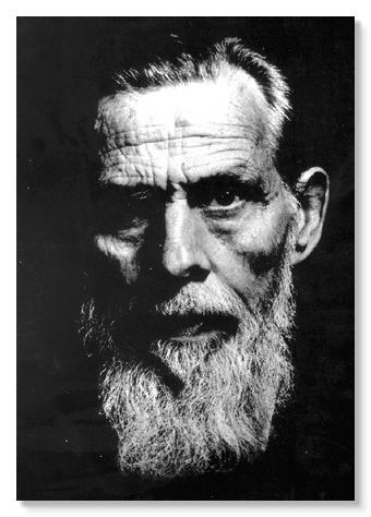
Figure: Donald M. MacKay (1922-1987), a physicist who was an early member of the cybernetics community and member of the Ratio Club.

Donald MacKay was a physicist who worked on naval gun targetting during the second world war. The challenge with gun targetting for ships is that both the target and the gun platform are moving. The challenge was tackled using analogue computers, for example in the US the Mark I fire control computer which was a mechanical computer. MacKay worked on radar systems for gun laying, here the velocity and distance of the target could be assessed through radar and an mechanical electrical analogue computer.

Fire Control Systems

Naval gunnery systems deal with targeting guns while taking into account movement of ships. The Royal Navy’s Gunnery Pocket Book (The Admiralty, 1945) gives details of one system for gun laying.

Like many challenges we face today, in the second world war, fire control was handled by a hybrid system of humans and computers. This means deploying human beings for the tasks that they can manage, and machines for the tasks that are better performed by a machine. This leads to a division of labour between the machine and the human that can still be found in our modern digital ecosystems.

Figure: The fire control computer set at the centre of a system of observation and tracking (The Admiralty, 1945).

As analogue computers, fire control computers from the second world war would contain components that directly represented the different variables that were important in the problem to be solved, such as the inclination between two ships.

Figure: Measuring inclination between two ships (The Admiralty, 1945). Sophisticated fire control computers allowed the ship to continue to fire while under maneuvers.

The fire control systems were electro-mechanical analogue computers that represented the “state variables” of interest, such as inclination and ship speed with gears and cams within the machine.

Figure: A second world war gun computer’s control table (The Admiralty, 1945).

For more details on fire control computers, you can watch a 1953 film on the the US the Mark IA fire control computer from Periscope Film.

Figure: U.S. Navy training film MN-6783a. Basic Mechanisms of Fire Control Computers. Mechanical Computer Instructional Film 27794 (1953) for the Mk 1A Fire Control Computer.

Behind the Eye

Figure: Behind the Eye (MacKay, 1991) summarises MacKay’s Gifford Lectures, where MacKay uses the operation of the eye as a window on the operation of the brain.

Donald MacKay was at King’s College for his PhD. He was just down the road from Bill Phillips at LSE who was building the MONIAC. He was part of the Ratio Club. A group of early career scientists who were interested in communication and control in animals and humans, or more specifically they were interested in computers and brains. The were part of an international movement known as cybernetics.

Donald MacKay wrote of the influence that his own work on radar had on his interest in the brain.

… during the war I had worked on the theory of automated and electronic computing and on the theory of information, all of which are highly relevant to such things as automatic pilots and automatic gun direction. I found myself grappling with problems in the design of artificial sense organs for naval gun-directors and with the principles on which electronic circuits could be used to simulate situations in the external world so as to provide goal-directed guidance for ships, aircraft, missiles and the like.

Later in the 1940’s, when I was doing my Ph.D. work, there was much talk of the brain as a computer and of the early digital computers that were just making the headlines as “electronic brains.” As an analogue computer man I felt strongly convinced that the brain, whatever it was, was not a digital computer. I didn’t think it was an analogue computer either in the conventional sense.

But this naturally rubbed under my skin the question: well, if it is not either of these, what kind of system is it? Is there any way of following through the kind of analysis that is appropriate to their artificial automata so as to understand better the kind of system the human brain is? That was the beginning of my slippery slope into brain research.

Behind the Eye pg 40. Edited version of the 1986 Gifford Lectures given by Donald M. MacKay and edited by Valerie MacKay

Importantly, MacKay distinguishes between the analogue computer and the digital computer. As he mentions, his experience was with analogue machines. An analogue machine is literally an analogue. The radar systems that Wiener and MacKay both worked on were made up of electronic components such as resistors, capacitors, inductors and/or mechanical components such as cams and gears. Together these components could represent a physical system, such as an anti-aircraft gun and a plane. The design of the analogue computer required the engineer to simulate the real world in analogue electronics, using dualities that exist between e.g. mechanical circuits (mass, spring, damper) and electronic circuits (inductor, resistor, capacitor). The analogy between mass and a damper, between spring and a resistor and between capacitor and a damper works because the underlying mathematics is approximated with the same linear system: a second order differential equation. This mathematical analogy allowed the designer to map from the real world, through mathematics, to a virtual world where the components reflected the real world through analogy.

This is a quite different from the approach that McCulloch and Pitts were taking with their paper on the logical calculus of the nervous system. They were attempting to map their model of the neuron onto logic. Logical reasoning was the mainstay of the contemporary understanding of intelligence. But the components they were considering were neurons, they could only map onto the logical world because their analogy for the neuron was so simple. An ‘on’ or ‘off’ linear threshold unit. Where the synapses of the neuron were compared to a threshold in the neuron. Firing occurs when the sum of input neurons crosses a threshold in the receiving neuron. These networks can then be built together in cascades.

Figure: A Colossus Mark 2 codebreaking computer being operated by Dorothy Du Boisson (left) and Elsie Booker (right). Colossus was designed by Tommy Flowers, but programmed and operated by groups of Wrens based at Bletchley Park.

In the late 1940s and early 1950s, Cyberneticists were also working on digital computers. The type of machines (such as Colossus, built by Tommy Flowers, and known to Turing) and the ENIAC. Indeed, by 1949 Cambridge had built its own machine, the EDSAC in the Mathematical Laboratory, inspired by “draft of a report on the EDVAC” by von Neumann.

Digital computers are themselves (at their heart) a series of analogue devices, but in the digital computer, the analogue is between collections of transistors and logic gates. Logic gates allow the computer to reconstruct logical truth tables, which Wittgenstein had popularised in his Tractatus Logico-Philosophicus (Wittgenstein, 1922). The mathematical operations we need can be reconstructed through logic, so this ‘analogue machine’ which we call a digital computer becomes capable of directly computing the mathematics we’re interested in, rather than going via the analogue machine.

The Perceptron

Figure: W. Ross Ashby (1903-1972), John von Neumann (1903-1957), Frank Rosenblatt (1928-1971). Photograph of W. Ross Ashby is Copyright W. Ross Ashby.

The early story of Cybernetics starts with the success of analogue control, and in the domain of neural networks, analogues machines were built. Inspired by F. Ross Ashby’s (Ashby, 1952) ideas that suggested random connections and von Neumann (Neumann, 1956), who wrote about probabilistic logics, Frank Rosenblatt constructed the Perceptron (Rosenblatt, 1958). This was a deep neural network that recognised images from TV cameras.

The perceptron created a great deal of interest, but it was rapidly eclipsed by the emerging digital computer. Perhaps as a marker as the increasing importance of the digital computer, the Apollo program (1961-1972) had a guidance computer that was a 16-bit digital machine for navigating to the moon. It implemented Kalman filters for guidance. In signal processing there’s a shift from the 1950s to the 1960s of researchers moving from analogue designs to designs that are suitable for implementation of digital machines.

That same shift was imposed on the Cybernetics community. Artificial Intelligence is often traced to the ‘summer research project’ proposed by John McCarthy at Dartmouth. But the proposal is not just notable for the introduction of the term, it is notable for the extent to which it marks a break with the Cybernetics community. Wiener’s name isn’t even mentioned in the proposal. And Cyberneticists either weren’t invited to, or couldn’t make, the event (with the notable exception of Warren McCulloch). Turing had died, and von Neumann was seriously ill with cancer. W. Ross Ashby was even in the US, but from his diaries there’s no trace of him attending. Donald MacKay was on the initial proposal, but didn’t make the event (perhaps because that summer his son, Robert, was born).

One of the great ironies of modern artificial intelligence is that it is almost wholly reliant on deep neural network methodologies for the recent breakthroughs. But the dawn of the term artificial intelligence is associated with a period of around three decades when those methods (and the community that originated them) was actively marginalised.

There were many reasons for this, including personal enmities between Wiener and McCulloch, the untimely death of Frank Rosenblatt in a sailing accident. But regardless of these personal tragedies and tales of academic politics, the principal reason that neural networks were eclipsed was the dominance of the digital computer. From 1956 to 1986 we saw the rise of the computer from a tool for science and big business to a personal machine, available to individual researchers.

The Connectionists

By the early 1980s, some disillusionment was creeping into the artificial intelligence agenda that stemmed from the Dartmouth Meeting. At the same time, an emerging group was re-examining the ideas of the Cyberneticists. This group became known as the connectionists, because of their focus on neural network models with their myriad of connections.

By the second half of the decade, some of their principles had come together to form a movement. Meetings including the Snowbird Workshop, Neural Information Processing Systems and the connectionist summer school provided a venue for these researchers to come together.

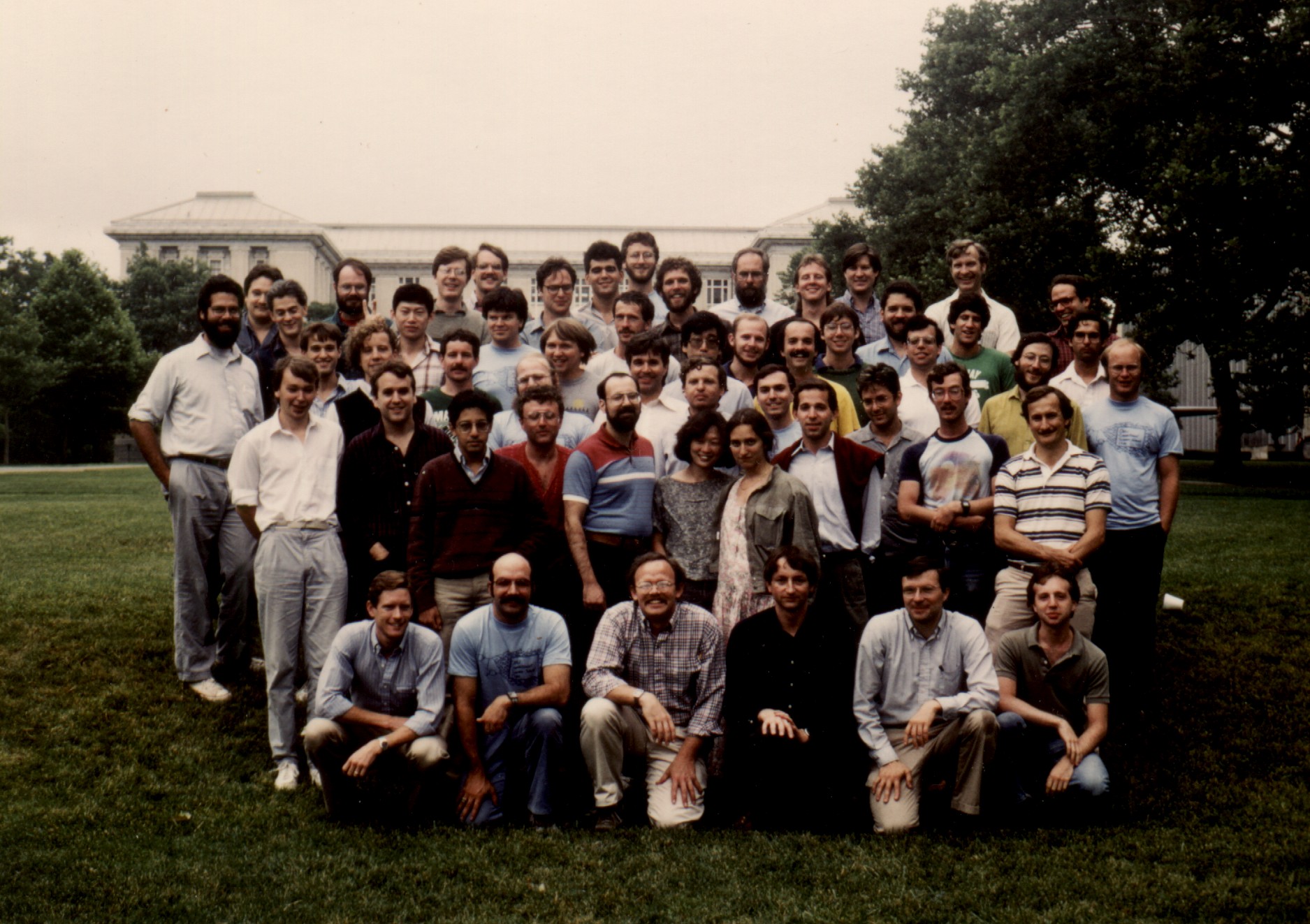
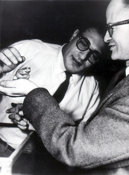
Figure: Group photo from the 1986 Connectionists’ Summer School, held at CMU in July. Included in the photo are Richard Durbin, Terry Sejnowski, Geoff Hinton, Yann LeCun, Michael I. Jordan.

This was also the era of cheap(er) computing. Connectionists were able to implement simulators of neural networks in minicomputers such as DEC’s PDP-11 series. These allowed new architectures to be tried. Among them was backpropagation, popularised by the “Parallel Distributed Processing” books (Rumelhart et al., 1986), these books formed the canonical ideas on which the connectionists based their research.

What makes people smarter than machines? They certainly are not quicker or more precise. Yet people are far better at perceiving objects in natural scenes and noting their relations, at understanding language and retrieving contextually appropriate information from memory, at making plans and carrying out contextually appropriate actions, and at a wide range of other natural cognitive tasks. People are also far better at learning to do these things more accurately and fluently through processing experience.

What is the basis for these differences? One answer, perhaps the classic one we might expect from artificial intelligence, is “software.” If we only had the right computer program, the argument goes, we might be able to capture the fluidity and adaptability of human information processing.

Certainly this answer is partially correct. There have been great breakthroughs in our understanding of cognition as a result of the development of expressive high-level computer languages and powerful algorithms. No doubt there will be more such breakthroughs in the future. However, we do not think that software is the whole story.

In our view, people are smarter than today’s computers because the brain employs a basic computational architecture that is more suited to deal with a central aspect of the natural information processing tasks that people are so good at.

J. L. McClelland, David E. Rumelhart and Geoffrey E. Hinton in Parallel Distributed Processing, Rumelhart et al. (1986)

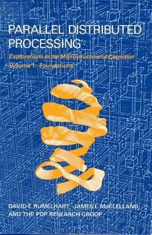
Figure: Cover of the Parallel Distributed Processing edited volume (Rumelhart et al., 1986).

This led to the second wave of neural network architectures. A new journal, Neural Computation was launched in 1989 to cater for this new field. It’s first volume contained a new architecture: the convolutional neural networks (Le Cun et al., 1989), developed for recognising handwritten digits. It made the cover.

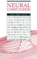
Figure: Cover of Neural Computation, Volume 1, Issue 4 containing Le Cun et al. (1989). The cover shows examples from the U.S. Postal Service data set of handwritten digits.

It’s worth noting what compute and data that LeCun and collaborators had available. Experiments were run on a SUN-4/260, with a CPU running at 16.67 MHz and 128 MB of RAM. It’s an impressive machine for the day. The neural network had just under 10,000 parameters and the training data consisted of 7,291 digitized training images on a 16 x 16 grid, 2007 images were retained for testing. The model had a 5% error rate on the test data.

The first several stages of processing in our previous system (described in Denker et al. 1989) involved convolutions in which the coefficients had been laboriously hand designed. In the present system, the first two layers of the network are constrained to be convolutional, but the system automatically learns the coefficients that make up the kernels.

Section 5.1 in Le Cun et al. (1989)

The second half of the 1980s and the 1990s were a period of growth and innovation for the community. Recurrent neural networks that operated through time were produced including in 1997, the Long Short-Term Memory architecture (Hochreiter and Schmidhuber, 1997), a form of recurrent neural network that can deal with sequence data.

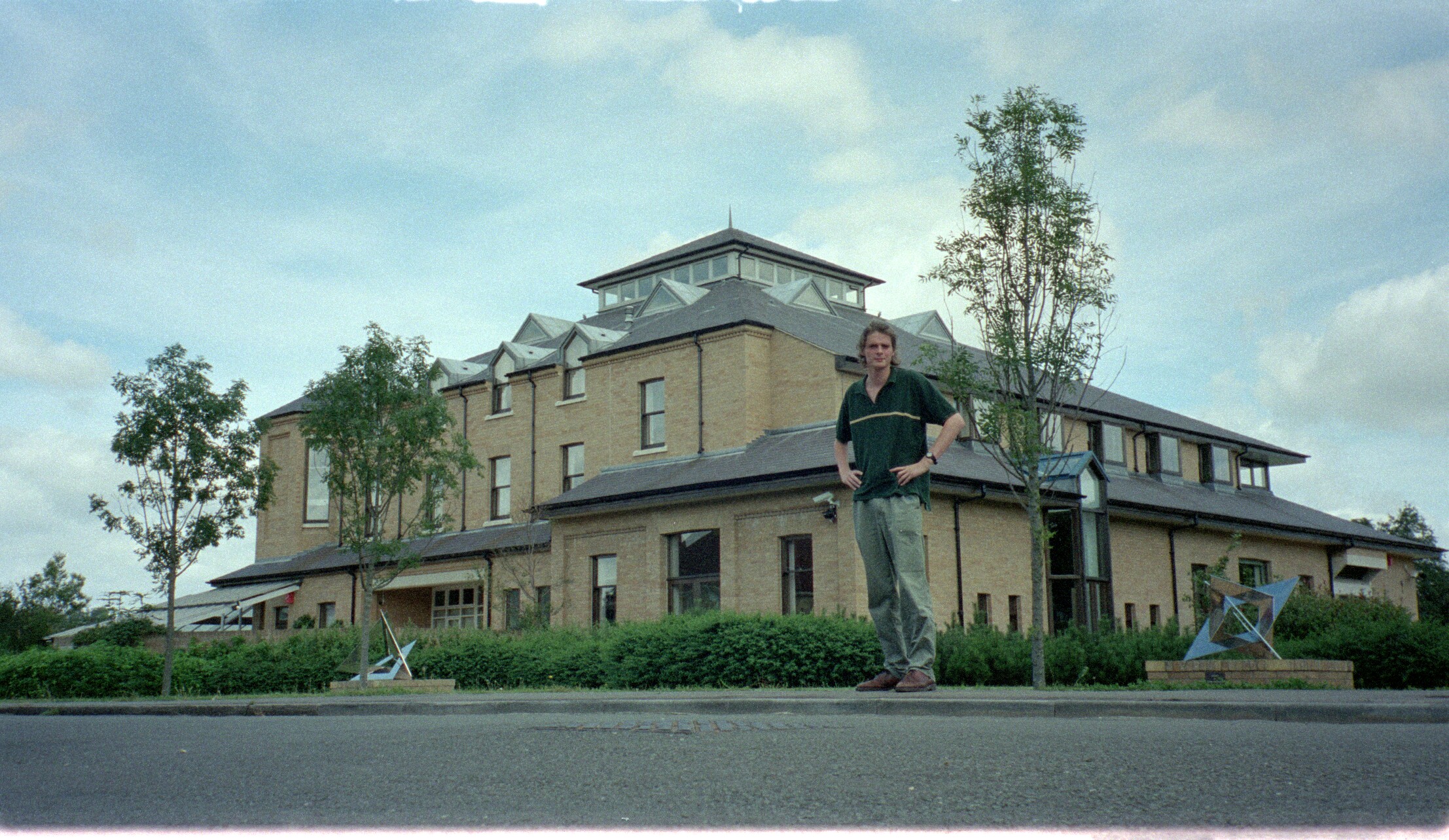
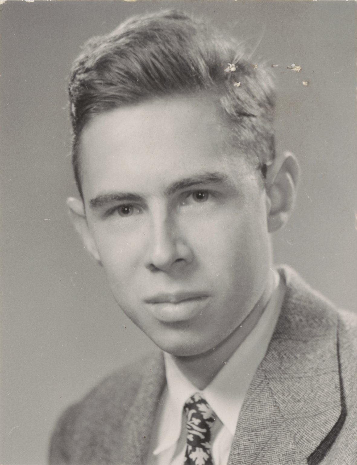
Figure: Neil standing outside the Newton Institute on 2nd August 1997, just after arriving for “Generalisation in Neural Networks and Machine Learning”, see page 26-30 of this report.

Figure: Gif animation of LeNet-5 in action.

Figure: Gif animation of LeNet-5 in action. Here the translation invariance of the network is being tested.

Figure: Gif animation of LeNet-5 in action, here the scale invariance of the network is being tested.

At the same meeting Vladmir Vapnik was present, as was Bernhard Schölkopf. Corinna Cortes, Bernard Boser, Isabelle Guyon and Vladmir Vapnik were all instrumental in developing the Support Vector Machine.

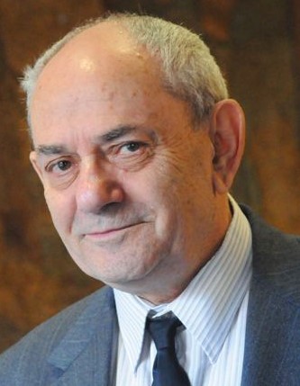
Figure: Corinna Cortes, Isabelle Guyon and Vladmir Vapnik. Three of the key people behind the support vector machine Cortes and Vapnik (1995). All were based at Bell Labs in the 1990s.

Also attending the summer school at the Newton Institute was Bernhard Schölkopf. He had shown that, on the same USPS digits data set, the support vector machine was able to achieve an error of 4.2% (Schölkopf et al., 1997). It was also mathematically more elegant than the neural network approaches. Even on larger data sets, by incorporating the translation invariance (Schölkopf et al., n.d.), the support vector machine was able to achieve similar error rates to convolutional neural networks.

This work points out the necessity of having flexible “network design” software tools that ease the design of complex, specialized network architectures

From conclusions of Le Cun et al. (1989)

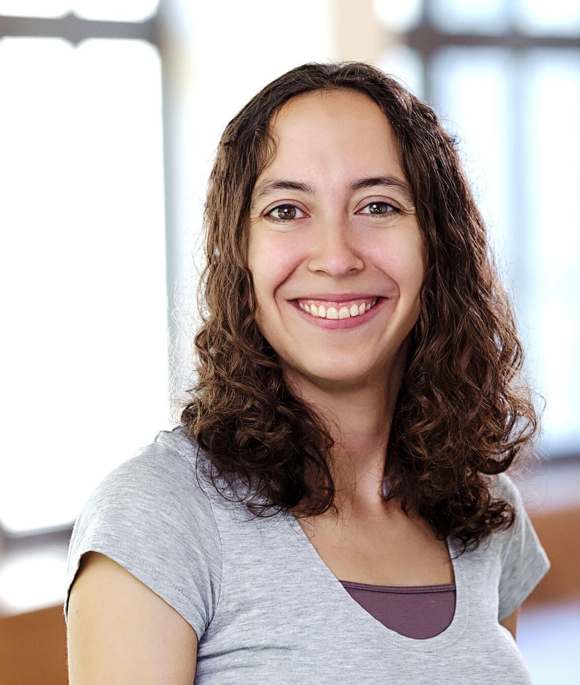
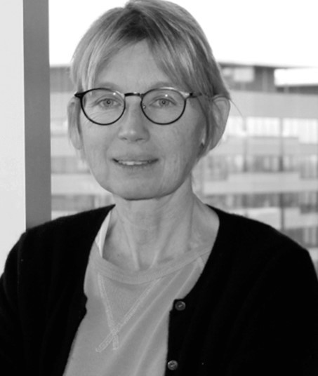
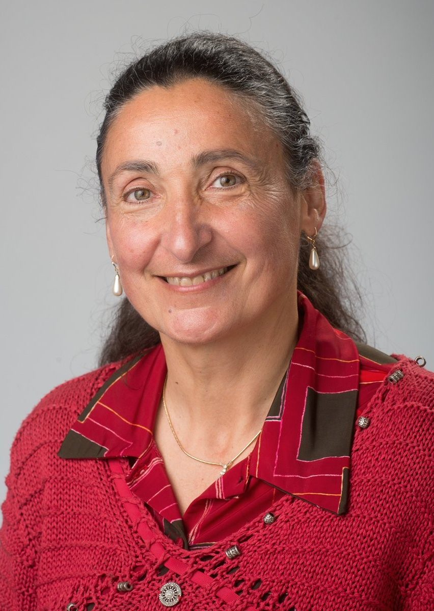
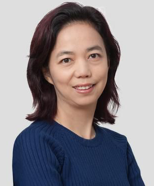
Figure: Olga Russakovsky, Fei Fei Li. Olga and Fei Fei led the creation of the ImageNet database that enabled convolutional neural networks to show their true potential. The data base contains millions of images.

The Third Wave

• Data (many data, many classes)
• Compute (GPUs)
• Stochastic Gradient Descent
• Software (autograd)

Domains of Use

• Perception and Representation
  1. Speech
  2. Vision
  3. Language

Experience

• Bringing it together:
  • Unsupervised pre-training
  • Initialisation and RELU
  • A Zoo of methods and models

• Why do they generalize well?

Conclusion

• Understand the principles behind:
  • Generalization
  • Optimization
  • Implementation (hardware)
• Different NN Architectures

Thanks!

For more information on these subjects and more you might want to check the following resources.

• twitter: @lawrennd
• podcast: The Talking Machines
• newspaper: Guardian Profile Page
• blog: http://inverseprobability.com

References