Week 6: Visualisation

[jupyter][google colab][reveal]

Neil D. Lawrence

Abstract:

In this lecture we turn to unsupervised learning. Specifically, we introduce the idea of a latent variable model. Latent variable models are a probabilistic perspective on unsupervised learning which lead to dimensionality reduction algorithms.

Setup

notutils

This small package is a helper package for various notebook utilities used below.

The software can be installed using

%pip install notutils

from the command prompt where you can access your python installation.

The code is also available on GitHub: https://github.com/lawrennd/notutils

Once notutils is installed, it can be imported in the usual manner.

import notutils

pods

In Sheffield we created a suite of software tools for ‘Open Data Science’. Open data science is an approach to sharing code, models and data that should make it easier for companies, health professionals and scientists to gain access to data science techniques.

You can also check this blog post on Open Data Science.

The software can be installed using

%pip install pods

from the command prompt where you can access your python installation.

The code is also available on GitHub: https://github.com/lawrennd/ods

Once pods is installed, it can be imported in the usual manner.

import pods

mlai

The mlai software is a suite of helper functions for teaching and demonstrating machine learning algorithms. It was first used in the Machine Learning and Adaptive Intelligence course in Sheffield in 2013.

The software can be installed using

%pip install mlai

from the command prompt where you can access your python installation.

The code is also available on GitHub: https://github.com/lawrennd/mlai

Once mlai is installed, it can be imported in the usual manner.

import mlai

Review

Last time with generalised linear models we focussed mainly on regression problems, which are examples of supervised learning. We have considered the relationship between the likelihood and the objective function and we have shown how we can find paramters by maximizing the likelihood (equivalent to minimizing the objective function) and in the last session we saw how we can marginalize the parameters in a process known as Bayesian inference.

Clustering

• One common approach, not deeply covered in this course.

• Associate each data point, \(\mathbf{ y}_{i, :}\) with one of \(k\) different discrete groups.

• For example:

  • Clustering animals into discrete groups. Are animals discrete or continuous?
  • Clustering into different different political affiliations.

• Humans do seem to like clusters:

  • Very useful when interacting with biologists.

• Subtle difference between clustering and vector quantisation

• Little anecdote.

• To my mind difference is in clustering there should be a reduction in data density between samples.

• This definition is not universally applied.

• For today’s purposes we merge them:

  • Determine how to allocate each point to a group and harder total number of groups.

• Simple algorithm for allocating points to groups.

• Require: Set of \(k\) cluster centres & assignment of each points to a cluster.

1. Initialize cluster centres as randomly selected data points.
   2. Assign each data point to nearest cluster centre.
   3. Update each cluster centre by setting it to the mean of assigned data points.
   4. Repeat 2 and 3 until cluster allocations do not change.

• This minimizes the objective \[ E=\sum_{j=1}^K \sum_{i\ \text{allocated to}\ j} \left(\mathbf{ y}_{i, :} - \boldsymbol{ \mu}_{j, :}\right)^\top\left(\mathbf{ y}_{i, :} - \boldsymbol{ \mu}_{j, :}\right) \] i.e. it minimizes thesum of Euclidean squared distances betwen points and their associated centres.
• The minimum is not guaranteed to be global or unique.
• This objective is a non-convex optimization problem.

Clustering methods associate each data point with a different label. Unlike in classification the label is not provided by a human annotator. It is allocated by the computer. Clustering is quite intuitive for humans, we do it naturally with our observations of the real world. For example, we cluster animals into different groups. If we encounter a new animal, we can immediately assign it to a group: bird, mammal, insect. These are certainly labels that can be provided by humans, but they were also originally invented by humans. With clustering we want the computer to recreate that process of inventing the label.

Unsupervised learning enables computers to form similar categorizations on data that is too large scale for us to process. When the Greek philosopher, Plato, was thinking about ideas, he considered the concept of the Platonic ideal. The Platonic ideal bird is the bird that is most bird-like or the chair that is most chair-like. In some sense, the task in clustering is to define different clusters, by finding their Platonic ideal (known as the cluster center) and allocate each data point to the relevant cluster center. So, allocate each animal to the class defined by its nearest cluster center.

To perform clustering on a computer we need to define a notion of either similarity or distance between the objects and their Platonic ideal, the cluster center. We normally assume that our objects are represented by vectors of data, \(\mathbf{ x}_i\). Similarly, we represent our cluster center for category \(j\) by a vector \(\boldsymbol{ \mu}_j\). This vector contains the ideal features of a bird, a chair, or whatever category \(j\) is. In clustering we can either think in terms of similarity of the objects, or distances. We want objects that are similar to each other to cluster together. We want objects that are distant from each other to cluster apart.

This requires us to formalize our notion of similarity or distance. Let’s focus on distances. A definition of distance between an object, \(i\), and the cluster center of class \(j\) is a function of two vectors, the data point, \(\mathbf{ x}_i\) and the cluster center, \(\boldsymbol{ \mu}_j\), \[ d_{ij} = f(\mathbf{ x}_i, \boldsymbol{ \mu}_j). \] Our objective is then to find cluster centers that are close to as many data points as possible. For example, we might want to cluster customers into their different tastes. We could represent each customer by the products they’ve purchased in the past. This could be a binary vector \(\mathbf{ x}_i\). We can then define a distance between the cluster center and the customer.

Squared Distance

A commonly used distance is the squared distance, \[ d_{ij} = (\mathbf{ x}_i - \boldsymbol{ \mu}_j)^2. \] The squared distance comes up a lot in machine learning. In unsupervised learning it was used to measure dissimilarity between predictions and observed data. Here its being used to measure the dissimilarity between a cluster center and the data.

Once we have decided on the distance or similarity function, we can decide a number of cluster centers, \(K\). We find their location by allocating each center to a sub-set of the points and minimizing the sum of the squared errors, \[ E(\mathbf{M}) = \sum_{i \in \mathbf{i}_j} (\mathbf{ x}_i - \boldsymbol{ \mu}_j)^2 \] where the notation \(\mathbf{i}_j\) represents all the indices of each data point which has been allocated to the \(j\)th cluster represented by the center \(\boldsymbol{ \mu}_j\).

\(k\)-Means Clustering

One approach to minimizing this objective function is known as \(k\)-means clustering. It is simple and relatively quick to implement, but it is an initialization sensitive algorithm. Initialization is the process of choosing an initial set of parameters before optimization. For \(k\)-means clustering you need to choose an initial set of centers. In \(k\)-means clustering your final set of clusters is very sensitive to the initial choice of centers. For more technical details on \(k\)-means clustering you can watch a video of Alex Ihler introducing the algorithm here.

\(k\)-Means Clustering

Figure: Clustering with the \(k\)-means clustering algorithm.

Figure: \(k\)-means clustering by Alex Ihler.

Hierarchical Clustering

Other approaches to clustering involve forming taxonomies of the cluster centers, like humans apply to animals, to form trees. You can learn more about agglomerative clustering in this video from Alex Ihler.

Figure: Hierarchical Clustering by Alex Ihler.

Phylogenetic Trees

Indeed, one application of machine learning techniques is performing a hierarchical clustering based on genetic data, i.e. the actual contents of the genome. If we do this across a number of species then we can produce a phylogeny. The phylogeny aims to represent the actual evolution of the species and some phylogenies even estimate the timing of the common ancestor between two species¹. Similar methods are used to estimate the origin of viruses like AIDS or Bird flu which mutate very quickly. Determining the origin of viruses can be important in containing or treating outbreaks.

Product Clustering

An e-commerce company could apply hierarchical clustering to all its products. That would give a phylogeny of products. Each cluster of products would be split into sub-clusters of products until we got down to individual products. For example, we might expect a high level split to be Electronics/Clothing. Of course, a challenge with these tree-like structures is that many products belong in more than one parent cluster: for example running shoes should be in more than one group, they are ‘sporting goods’ and they are ‘apparel’. A tree structure doesn’t allow this allocation.

Hierarchical Clustering Challenge

Our own psychological grouping capabilities are studied as a domain of cognitive science. Researchers like Josh Tenenbaum have developed algorithms that decompose data in more complex ways, but they can normally only be applied to smaller data sets.

Other Clustering Approaches

• Spectral clustering (Shi and Malik (2000),Ng et al. (n.d.))
  • Allows clusters which aren’t convex hulls.
• Dirichlet process
  • A probabilistic formulation for a clustering algorithm that is non-parametric.
  • Loosely speaking it allows infinite clusters
  • In practice useful for dealing with previously unknown species (e.g. a “Black Swan Event”).

High Dimensional Data

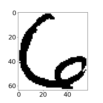
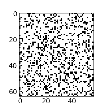
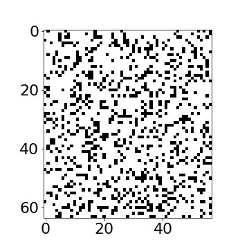
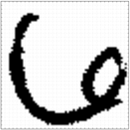
To introduce high dimensional data, we will first of all introduce a hand written digit from the U.S. Postal Service handwritten digit data set (originally collected from scanning enveolopes) and used in the first convolutional neural network paper (Le Cun et al., 1989).

Le Cun et al. (1989) downscaled the images to \(16 \times 16\), here we use an image at the original scale, containing 64 rows and 57 columns. Since the pixels are binary, and the number of dimensions is 3,648, this space contains \(2^{3,648}\) possible images. So this space contains a lot more than just one digit.

USPS Samples

If we sample from this space, taking each pixel independently from a probability which is given by the number of pixels which are ‘on’ in the original image, over the total number of pixels, we see images that look nothing like the original digit.

Figure: Even if we sample every nano second from now until the end of the universe we won’t see the original six again.

Even if we sample every nanosecond from now until the end of the universe you won’t see the original six again.

Simple Model of Digit

So, an independent pixel model for this digit doesn’t seem sensible. The total space is enormous, and yet the space occupied by the type of data we’re interested in is relatively small.

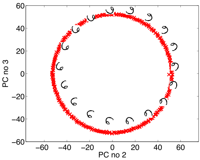
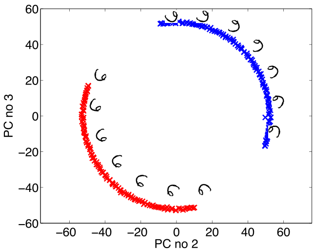
Consider a different type of model. One where we take a prototype six and we rotate it left and right to create new data.

%pip install scikit-image

Figure: Rotate a prototype six to form a set of plausible sixes.

Figure: The rotated sixes projected onto the first two principal components of the ‘rotated data set’. The data lives on a one dimensional manifold in the 3,648 dimensional space.

Low Dimensional Manifolds

Of course, in practice pure rotation of the image is too simple a model. Digits can undergo several distortions and retain their nature. For example, they can be scaled, they can go through translation, they can udnergo ‘thinning’. But, for data with ‘structure’ we expect fewer of these distortions than the dimension of the data. This means we expect data to live on a lower dimensonal manifold. This implies that we should deal with high dimensional data by looking for a lower dimensional (non-linear) embedding.

Latent Variables

Latent means hidden, and hidden variables are simply unobservable variables. The idea of a latent variable is crucial to the concept of artificial intelligence, machine learning and experimental design. A latent variable could take many forms. We might observe a man walking along a road with a large bag of clothes and we might infer that the man is walking to the laundrette. Our observations are a highly complex data space, the response in our eyes is processed through our visual cortex, the combination of the individual’s limb movememnts and the direction they are walking in all conflate in our heads to cause us to infer that (perhaps) the individual is going to the laundrette. We don’t know that the man is walking to the laundrette, but we have a model of the world that suggests that it’s a likely outcome for the very complex data. In some ways the latent variable can be seen as a compression of this very complex scene. If I were writing a book, I might write that “A man tripped over whilst walking to the laundrette”. In the reader’s mind an image of a man, perhaps laden with dirty clothes, may occur. All these ideas come from our expectations of the world around us. We can make further inference about the man, some of it perhaps plausible others less so. The man may be going to the laundrette because his washing machine is broken, or because he doesn’t have a large enough flat to have a washing machine, or because he’s carrying a duvet, or because he doesn’t like ironing. All of these may increase in probability given our observation, but they are still latent variables. Unless we follow the man back to his appartment, or start making other enquirires about the man, we don’t know the true answer.

It’s clear that to do inference about any complex system we must include latent variables. Latent variables are extremely powerful. In robotics, they are used to represent the state of the robot. The state of the robot may include its position (in x, y coordinates) its speed, its direction of facing. How are these variables unknown to the robot? Well the robot only posesses sensors, it can make observations of the nearest object in a certain direction, and it may have a map of its environment. If we represent the state of the robot as its position on a map, it may be uncertain of that position. If you go walking or running in the hills around Sheffield, you can take a very high quality ordnance survey map with you. However, unless you are a really excellent orienteer, when you are far from any given landmark, you will probably be uncertain about your true position on the map. These states are also latent variables.

In statistical analysis of experiments you try to control for each aspect of the experiment, in particular by randomization. So if I’m interested in the ability of a particular fertilizer to improve the yield of a particular plant I may design an experiment where I apply the fertilizer to some plants (the treatment group) and withold the fertilizer from others (the control group). I then test to see whether the yield from the treatment group is better (or worse) than the control group. I may find that I have an excellent yield for the treatment group. However, what if I’d (unknowlingly) planted all my treatment plants in a sunny part of the field, and all the control plants in a shady part of the field. That would also be a latent variable, in this case known as a confounder. In statistical experimental design randomization is used to attempt to eliminate the correlated effects of these confounders: you aim to ensure that if these confounders do exist their effects are not correlated with treatment and contorl. This is known as a randomized control trial.

Greek philosophers worried a great deal about what was knowable and what was unknowable. Adherents of philosophical Skeptisism were inspired by the idea that since your senses sometimes give you contradictory information, they cannot be trusted, and in extreme cases they chose to ignore their senses. This is an acknowledgement that very often the true state of the world cannot be known with precision. Unfortunately, these philosophers didn’t have a good understanding of probability, so they were unable to encapsulate their ideas through a degree of belief.

We often use language to express the compression of a complex behavior or patterns in a simpler way, for example we talk about motives as a useful distallation for a perhaps very complex patter of behavior. In physics we use principles of causation and simple laws to describe the world around us. Such motives or underlying principles are difficult to observe directly, our conclusions about them emerge over a period of time by observing indirect consequences of the latent variables.

Epistemic uncertainty allows us to deal with these worries by associating our degree of belief about the state of the world with a probaiblity distribution. This core idea underpins state space modelling, probabilistic graphical models and the wider field of latent variable modelling. In this session we are going to explore the idea in a simple linear system and see how it relates to factor analysis and principal component analysis.

Your Personality

At the beginning of the 20th century there was a great deal of interest amoungst psychologists in formalizing patterns of thought. The approach they used became known as factor analysis. The principle is that we observe a potentially high dimensional vector of characteristics about an individual. To formalize this, social scientists designed questionaires. We can envisage many questions that we may ask, but the assumption is that underlying these questions there are only a few traits that dictate the behavior. These models are known as latent trait models and the analysis is sometimes known as factor analysis. The idea is that there are a few characteristic traits that we are looking to discern. These traits or factors can be extracted by assimilating the high dimensional characteristics of the individual into a few latent factors.

Factor Analysis Model

This causes us to consider a model as follows, if we are given a high dimensional vector of features (perhaps questionaire answers) associated with an individual, \(\mathbf{ y}\), we assume that these factors are actually generated from a low dimensional vector latent traits, or latent variables, which determine the personality. \[ \mathbf{ y}= \mathbf{f}(\mathbf{ z}) + \boldsymbol{ \epsilon}, \] where \(\mathbf{f}(\mathbf{ z})\) is a vector valued function that is dependent on the latent traits and \(\boldsymbol{ \epsilon}\) is some corrupting noise. For simplicity, we assume that the function is given by a linear relationship, \[ \mathbf{f}(\mathbf{ z}) = \mathbf{W}\mathbf{ z} \] where we have introduced a matrix \(\mathbf{W}\) that is sometimes referred to as the factor loadings but we also immediately see is related to our multivariate linear regression models from the . That is because our vector valued function is of the form

\[ \mathbf{f}(\mathbf{ z}) = \begin{bmatrix} f_1(\mathbf{ z}) \\ f_2(\mathbf{ z}) \\ \vdots \\ f_p(\mathbf{ z})\end{bmatrix} \] where there are \(p\) features associated with the individual. If we consider any of these functions individually we have a prediction function that looks like a regression model, \[ f_j(\mathbf{ z}) = \mathbf{ w}_{j, :}^\top \mathbf{ z}, \] for each element of the vector valued function, where \(\mathbf{ w}_{:, j}\) is the \(j\)th column of the matrix \(\mathbf{W}\). In that context each column of \(\mathbf{W}\) is a vector of regression weights. This is a multiple input and multiple output regression. Our inputs (or covariates) have dimensionality greater than 1 and our outputs (or response variables) also have dimensionality greater than one. Just as in a standard regression, we are assuming that we don’t observe the function directly (note that this also makes the function a type of latent variable), but we observe some corrupted variant of the function, where the corruption is given by \(\boldsymbol{ \epsilon}\). Just as in linear regression we can assume that this corruption is given by Gaussian noise, where the noise for the \(j\)th element of \(\mathbf{ y}\) is by, \[ \epsilon_j \sim \mathcal{N}\left(0,\sigma^2_j\right). \] Of course, just as in a regression problem we also need to make an assumption across the individual data points to form our full likelihood. Our data set now consists of many observations of \(\mathbf{ y}\) for diffetent individuals. We store these observations in a design matrix, \(\mathbf{Y}\), where each row of \(\mathbf{Y}\) contains the observation for one individual. To emphasize that \(\mathbf{ y}\) is a vector derived from a row of \(\mathbf{Y}\) we represent the observation of the features associated with the \(i\)th individual by \(\mathbf{ y}_{i, :}\), and place each individual in our data matrix,

\[ \mathbf{Y} = \begin{bmatrix} \mathbf{ y}_{1, :}^\top \\ \mathbf{ y}_{2, :}^\top \\ \vdots \\ \mathbf{ y}_{n, :}^\top\end{bmatrix}, \] where we have \(n\) data points. Our data matrix therefore has \(n\) rows and \(p\) columns. The point to notice here is that each data obsesrvation appears as a row vector in the design matrix (thus the transpose operation inside the brackets). Our prediction functions are now actually a matrix value function, \[ \mathbf{F} = \mathbf{Z}\mathbf{W}^\top, \] where for each matrix the data points are in the rows and the data features are in the columns. This implies that if we have \(q\) inputs to the function we have \(\mathbf{F}\in \Re^{n\times p}\), \(\mathbf{W}\in \Re^{p \times q}\) and \(\mathbf{Z}\in \Re^{n\times q}\).

Exercise 1

Show that, given all the definitions above, if, \[ \mathbf{F} = \mathbf{Z}\mathbf{W}^\top \] and the elements of the vector valued function \(\mathbf{F}\) are given by \[ f_{i, j} = f_j(\mathbf{ z}_{i, :}), \] where \(\mathbf{ z}_{i, :}\) is the \(i\)th row of the latent variables, \(\mathbf{Z}\), then show that \[ f_j(\mathbf{ z}_{i, :}) = \mathbf{ w}_{j, :}^\top \mathbf{ z}_{i, :} \]

Latent Variables vs Linear Regression

The difference between this model and a multiple output regression is that in the regression case we are provided with the covariates \(\mathbf{Z}\), here they are latent variables. These variables are unknown. Just as we have done in the past for unknowns, we now treat them with a probability distribution. In factor analysis we assume that the latent variables have a Gaussian density which is independent across both across the latent variables associated with the different data points, and across those associated with different data features, so we have, \[ x_{i,j} \sim \mathcal{N}\left(0,1\right), \] and we can write the density governing the latent variable associated with a single point as, \[ \mathbf{ z}_{i, :} \sim \mathcal{N}\left(\mathbf{0},\mathbf{I}\right). \] If we consider the values of the function for the \(i\)th data point as \[ \mathbf{f}_{i, :} = \mathbf{f}(\mathbf{ z}_{i, :}) = \mathbf{W}\mathbf{ z}_{i, :} \] then we can use the rules for multivariate Gaussian relationships to write that \[ \mathbf{f}_{i, :} \sim \mathcal{N}\left(\mathbf{0},\mathbf{W}\mathbf{W}^\top\right) \] which implies that the distribution for \(\mathbf{ y}_{i, :}\) is given by \[ \mathbf{ y}_{i, :} = \sim \mathcal{N}\left(\mathbf{0},\mathbf{W}\mathbf{W}^\top + \boldsymbol{\Sigma}\right) \] where \(\boldsymbol{\Sigma}\) the covariance of the noise variable, \(\epsilon_{i, :}\) which for factor analysis is a diagonal matrix (because we have assumed that the noise was independent across the features), \[ \boldsymbol{\Sigma} = \begin{bmatrix}\sigma^2_{1} & 0 & 0 & 0\\ 0 & \sigma^2_{2} & 0 & 0\\ 0 & 0 & \ddots & 0\\ 0 & 0 & 0 & \sigma^2_p\end{bmatrix}. \] For completeness, we could also add in a mean for the data vector \(\boldsymbol{ \mu}\), \[ \mathbf{ y}_{i, :} = \mathbf{W}\mathbf{ z}_{i, :} + \boldsymbol{ \mu}+ \boldsymbol{ \epsilon}_{i, :} \] which would give our marginal distribution for \(\mathbf{ y}_{i, :}\) a mean \(\boldsymbol{ \mu}\). However, the maximum likelihood solution for \(\boldsymbol{ \mu}\) turns out to equal the empirical mean of the data, \[ \boldsymbol{ \mu}= \frac{1}{n} \sum_{i=1}^n \mathbf{ y}_{i, :}, \] regardless of the form of the covariance, \(\mathbf{C}= \mathbf{W}\mathbf{W}^\top + \boldsymbol{\Sigma}\). As a result it is very common to simply preprocess the data and ensure it is zero mean. We will follow that convention for this session.

The prior density over latent variables is independent, and the likelihood is independent, that means that the marginal likelihood here is also independent over the data points. Factor analysis was developed mainly in psychology and the social sciences for understanding personality and intelligence. Charles Spearman was concerned with the measurements of “the abilities of man” and is credited with the earliest version of factor analysis.

Principal Component Analysis

In 1933 Harold Hotelling published on principal component analysis the first mention of this approach (Hotelling, 1933). Hotelling’s inspiration was to provide mathematical foundation for factor analysis methods that were by then widely used within psychology and the social sciences. His model was a factor analysis model, but he considered the noiseless ‘limit’ of the model. In other words he took \(\sigma^2_i \rightarrow 0\) so that he had

\[ \mathbf{ y}_{i, :} \sim \lim_{\sigma^2 \rightarrow 0} \mathcal{N}\left(\mathbf{0},\mathbf{W}\mathbf{W}^\top + \sigma^2 \mathbf{I}\right). \] The paper had two unfortunate effects. Firstly, the resulting model is no longer valid probablistically, because the covariance of this Gaussian is ‘degenerate’. Because \(\mathbf{W}\mathbf{W}^\top\) has rank of at most \(q\) where \(q<p\) (due to the dimensionality reduction) the determinant of the covariance is zero, meaning the inverse doesn’t exist so the density, \[ p(\mathbf{ y}_{i, :}|\mathbf{W}) = \lim_{\sigma^2 \rightarrow 0} \frac{1}{(2\pi)^\frac{p}{2} |\mathbf{W}\mathbf{W}^\top + \sigma^2 \mathbf{I}|^{\frac{1}{2}}} \exp\left(-\frac{1}{2}\mathbf{ y}_{i, :}\left[\mathbf{W}\mathbf{W}^\top+ \sigma^2 \mathbf{I}\right]^{-1}\mathbf{ y}_{i, :}\right), \] is not valid for \(q<p\) (where \(\mathbf{W}\in \Re^{p\times q}\)). This mathematical consequence is a probability density which has no ‘support’ in large regions of the space for \(\mathbf{ y}_{i, :}\). There are regions for which the probability of \(\mathbf{ y}_{i, :}\) is zero. These are any regions that lie off the hyperplane defined by mapping from \(\mathbf{ z}\) to \(\mathbf{ y}\) with the matrix \(\mathbf{W}\). In factor analysis the noise corruption, \(\boldsymbol{ \epsilon}\), allows for points to be found away from the hyperplane. In Hotelling’s PCA the noise variance is zero, so there is only support for points that fall precisely on the hyperplane. Secondly, Hotelling explicity chose to rename factor analysis as principal component analysis, arguing that the factors social scientist sought were different in nature to the concept of a mathematical factor. This was unfortunate because the factor loadings, \(\mathbf{W}\) can also be seen as factors in the mathematical sense because the model Hotelling defined is a Gaussian model with covariance given by \(\mathbf{C}= \mathbf{W}\mathbf{W}^\top\) so \(\mathbf{W}\) is a factor of the covariance in the mathematical sense, as well as a factor loading.

However, the paper had one great advantage over standard approaches to factor analysis. Despite the fact that the model was a special case that is subsumed by the more general approach of factor analysis it is this special case that leads to a particular algorithm, namely that the factor loadings (or principal components as Hotelling referred to them) are given by an eigenvalue decomposition of the empirical covariance matrix.

Computation of the Marginal Likelihood

\[ \mathbf{ y}_{i,:}=\mathbf{W}\mathbf{ z}_{i,:}+\boldsymbol{ \epsilon}_{i,:},\quad \mathbf{ z}_{i,:} \sim \mathcal{N}\left(\mathbf{0},\mathbf{I}\right), \quad \boldsymbol{ \epsilon}_{i,:} \sim \mathcal{N}\left(\mathbf{0},\sigma^{2}\mathbf{I}\right) \]

\[ \mathbf{W}\mathbf{ z}_{i,:} \sim \mathcal{N}\left(\mathbf{0},\mathbf{W}\mathbf{W}^\top\right) \]

\[ \mathbf{W}\mathbf{ z}_{i, :} + \boldsymbol{ \epsilon}_{i, :} \sim \mathcal{N}\left(\mathbf{0},\mathbf{W}\mathbf{W}^\top + \sigma^2 \mathbf{I}\right) \]

Probabilistic PCA Max. Likelihood Soln (Tipping and Bishop (1999a))

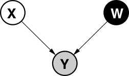
Figure: Graphical model representing probabilistic PCA.

\[p\left(\mathbf{Y}|\mathbf{W}\right)=\prod_{i=1}^{n}\mathcal{N}\left(\mathbf{ y}_{i, :}|\mathbf{0},\mathbf{W}\mathbf{W}^{\top}+\sigma^{2}\mathbf{I}\right)\]

Eigenvalue Decomposition

Eigenvalue problems are widespreads in physics and mathematics, they are often written as a matrix/vector equation but we prefer to write them as a full matrix equation. In an eigenvalue problem you are looking to find a matrix of eigenvectors, \(\mathbf{U}\) and a diagonal matrix of eigenvalues, \(\boldsymbol{\Lambda}\) that satisfy the matrix equation \[ \mathbf{A}\mathbf{U} = \mathbf{U}\boldsymbol{\Lambda}. \] where \(\mathbf{A}\) is your matrix of interest. This equation is not trivially solvable through matrix inverse because matrix multiplication is not commutative, so premultiplying by \(\mathbf{U}^{-1}\) gives \[ \mathbf{U}^{-1}\mathbf{A}\mathbf{U} = \boldsymbol{\Lambda}, \] where we remember that \(\boldsymbol{\Lambda}\) is a diagonal matrix, so the eigenvectors can be used to diagonalise the matrix. When performing the eigendecomposition on a Gaussian covariances, diagonalisation is very important because it returns the covariance to a form where there is no correlation between points.

Positive Definite

We are interested in the case where \(\mathbf{A}\) is a covariance matrix, which implies it is positive definite. A positive definite matrix is one for which the inner product, \[ \mathbf{ w}^\top \mathbf{C}\mathbf{ w} \] is positive for all values of the vector \(\mathbf{ w}\) other than the zero vector. One way of creating a positive definite matrix is to assume that the symmetric and positive definite matrix \(\mathbf{C}\in \Re^{p\times p}\) is factorised into, \(\mathbf{A}in \Re^{p\times p}\), a full rank matrix, so that \[ \mathbf{C}= \mathbf{A}^\top \mathbf{A}. \] This ensures that \(\mathbf{C}\) must be positive definite because \[ \mathbf{ w}^\top \mathbf{C}\mathbf{ w}=\mathbf{ w}^\top \mathbf{A}^\top\mathbf{A}\mathbf{ w} \] and if we now define a new vector \(\mathbf{b}\) as \[ \mathbf{b} = \mathbf{A}\mathbf{ w} \] we can now rewrite as \[ \mathbf{ w}^\top \mathbf{C}\mathbf{ w}= \mathbf{b}^\top\mathbf{b} = \sum_{i} b_i^2 \] which, since it is a sum of squares, is positive or zero. The constraint that \(\mathbf{A}\) must be full rank ensures that there is no vector \(\mathbf{ w}\), other than the zero vector, which causes the vector \(\mathbf{b}\) to be all zeros.

Exercise 2

If \(\mathbf{C}=\mathbf{A}^\top \mathbf{A}\) then express \(c_{i,j}\), the value of the element at the \(i\)th row and the \(j\)th column of \(\mathbf{C}\), in terms of the columns of \(\mathbf{A}\). Use this to show that (i) the matrix is symmetric and (ii) the matrix has positive elements along its diagonal.

Eigenvectors of a Symmetric Matric

Symmetric matrices have orthonormal eigenvectors. This means that \(\mathbf{U}\) is an orthogonal matrix, \(\mathbf{U}^\top\mathbf{U} = \mathbf{I}\). This implies that \(\mathbf{u}_{:, i} ^\top \mathbf{u}_{:, j}\) is equal to 0 if \(i\neq j\) and 1 if \(i=j\).

Principal Component Analysis

• PCA (Hotelling (1933)) is a linear embedding.

• Today its presented as:

  • Rotate to find ‘directions’ in data with maximal variance.
  • How do we find these directions?

• Algorithmically we do this by diagonalizing the sample covariance matrix \[ \mathbf{S}=\frac{1}{n}\sum_{i=1}^n\left(\mathbf{ y}_{i, :}-\boldsymbol{ \mu}\right)\left(\mathbf{ y}_{i, :} - \boldsymbol{ \mu}\right)^\top \]

• Find directions in the data, \(\mathbf{ z}= \mathbf{U}\mathbf{ y}\), for which variance is maximized.

• Solution is found via constrained optimisation (which uses Lagrange multipliers): \[ L\left(\mathbf{u}_{1},\lambda_{1}\right)=\mathbf{u}_{1}^{\top}\mathbf{S}\mathbf{u}_{1}+\lambda_{1}\left(1-\mathbf{u}_{1}^{\top}\mathbf{u}_{1}\right) \]

• Gradient with respect to \(\mathbf{u}_{1}\) \[\frac{\text{d}L\left(\mathbf{u}_{1},\lambda_{1}\right)}{\text{d}\mathbf{u}_{1}}=2\mathbf{S}\mathbf{u}_{1}-2\lambda_{1}\mathbf{u}_{1}\] rearrange to form \[\mathbf{S}\mathbf{u}_{1}=\lambda_{1}\mathbf{u}_{1}.\] Which is known as an eigenvalue problem.

• Further directions that are orthogonal to the first can also be shown to be eigenvectors of the covariance.

• Represent data, \(\mathbf{Y}\), with a lower dimensional set of latent variables \(\mathbf{Z}\).

• Assume a linear relationship of the form \[ \mathbf{ y}_{i,:}=\mathbf{W}\mathbf{ z}_{i,:}+\boldsymbol{ \epsilon}_{i,:}, \] where \[ \boldsymbol{ \epsilon}_{i,:} \sim \mathcal{N}\left(\mathbf{0},\sigma^2\mathbf{I}\right) \]

Probabilistic PCA

Define linear-Gaussian relationship between latent variables and data. Standard Latent variable approach: Define Gaussian prior over latent space, \(\mathbf{Z}\). Integrate out latent variables.

Figure: Graphical model representing probabilistic PCA. \[ p\left(\mathbf{Y}|\mathbf{Z},\mathbf{W}\right)=\prod_{i=1}^{n}\mathcal{N}\left(\mathbf{ y}_{i,:}|\mathbf{W}\mathbf{ z}_{i,:},\sigma^2\mathbf{I}\right) \] \[ p\left(\mathbf{Z}\right)=\prod_{i=1}^{n}\mathcal{N}\left(\mathbf{ z}_{i,:}|\mathbf{0},\mathbf{I}\right) \] \[ p\left(\mathbf{Y}|\mathbf{W}\right)=\prod_{i=1}^{n}\mathcal{N}\left(\mathbf{ y}_{i,:}|\mathbf{0},\mathbf{W}\mathbf{W}^{\top}+\sigma^{2}\mathbf{I}\right) \]

Probabilistic PCA

In 1997 Tipping and Bishop (Tipping and Bishop, 1999b) and Roweis (Roweis, n.d.) independently revisited Hotelling’s model and considered the case where the noise variance was finite, but shared across all output dimensons. Their model can be thought of as a factor analysis where \[ \boldsymbol{\Sigma} = \sigma^2 \mathbf{I}. \] This leads to a marginal likelihood of the form \[ p(\mathbf{Y}|\mathbf{W}, \sigma^2) = \prod_{i=1}^n\mathcal{N}\left(\mathbf{ y}_{i, :}|\mathbf{0},\mathbf{W}\mathbf{W}^\top + \sigma^2 \mathbf{I}\right) \] where the limit of \(\sigma^2\rightarrow 0\) is not taken. This defines a proper probabilistic model. Tippping and Bishop then went on to prove that the maximum likelihood solution of this model with respect to \(\mathbf{W}\) is given by an eigenvalue problem. In the probabilistic PCA case the eigenvalues and eigenvectors are given as follows. \[ \mathbf{W}= \mathbf{U}\mathbf{L} \mathbf{R}^\top \] where \(\mathbf{U}\) is the eigenvectors of the empirical covariance matrix \[ \mathbf{S} = \sum_{i=1}^n(\mathbf{ y}_{i, :} - \boldsymbol{ \mu})(\mathbf{ y}_{i, :} - \boldsymbol{ \mu})^\top, \] which can be written \(\mathbf{S} = \frac{1}{n} \mathbf{Y}^\top\mathbf{Y}\) if the data is zero mean. The matrix \(\mathbf{L}\) is diagonal and is dependent on the eigenvalues of \(\mathbf{S}\), \(\boldsymbol{\Lambda}\). If the \(i\)th diagonal element of this matrix is given by \(\lambda_i\) then the corresponding element of \(\mathbf{L}\) is \[ \ell_i = \sqrt{\lambda_i - \sigma^2} \] where \(\sigma^2\) is the noise variance. Note that if \(\sigma^2\) is larger than any particular eigenvalue, then that eigenvalue (along with its corresponding eigenvector) is discarded from the solution.

Python Implementation of Probabilistic PCA

We will now implement this algorithm in python.

import numpy as np

# probabilistic PCA algorithm
def ppca(Y, q):
    # remove mean
    Y_cent = Y - Y.mean(0)

    # Comute covariance
    S = np.dot(Y_cent.T, Y_cent)/Y.shape[0]
    lambd, U = np.linalg.eig(S)

    # Choose number of eigenvectors
    sigma2 = np.sum(lambd[q:])/(Y.shape[1]-q)
    l = np.sqrt(lambd[:q]-sigma2)
    W = U[:, :q]*l[None, :]
    return W, sigma2

In practice we may not wish to compute the eigenvectors of the covariance matrix directly. This is because it requires us to estimate the covariance, which involves a sum of squares term, before estimating the eigenvectors. We can estimate the eigenvectors directly either through QR decomposition or singular value decomposition. We saw a similar issue arise when , where we also wished to avoid computation of \(\mathbf{Z}^\top\mathbf{Z}\) (or in the case of \(\boldsymbol{\Phi}^\top\boldsymbol{\Phi}\)).

Posterior for Principal Component Analysis

Under the latent variable model justification for principal component analysis, we are normally interested in inferring something about the latent variables given the data. This is the distribution, \[ p(\mathbf{ z}_{i, :} | \mathbf{ y}_{i, :}) \] for any given data point. Determining this density turns out to be very similar to the approach for determining the Bayesian posterior of \(\mathbf{ w}\) in Bayesian linear regression, only this time we place the prior density over \(\mathbf{ z}_{i, :}\) instead of \(\mathbf{ w}\). The posterior is proportional to the joint density as follows, \[ p(\mathbf{ z}_{i, :} | \mathbf{ y}_{i, :}) \propto p(\mathbf{ y}_{i, :}|\mathbf{W}, \mathbf{ z}_{i, :}, \sigma^2) p(\mathbf{ z}_{i, :}) \] And as in the Bayesian linear regression case we first consider the log posterior, \[ \log p(\mathbf{ z}_{i, :} | \mathbf{ y}_{i, :}) = \log p(\mathbf{ y}_{i, :}|\mathbf{W}, \mathbf{ z}_{i, :}, \sigma^2) + \log p(\mathbf{ z}_{i, :}) + \text{const} \] where the constant is not dependent on \(\mathbf{ z}\). As before we collect the quadratic terms in \(\mathbf{ z}_{i, :}\) and we assemble them into a Gaussian density over \(\mathbf{ z}\). \[ \log p(\mathbf{ z}_{i, :} | \mathbf{ y}_{i, :}) = -\frac{1}{2\sigma^2} (\mathbf{ y}_{i, :} - \mathbf{W}\mathbf{ z}_{i, :})^\top(\mathbf{ y}_{i, :} - \mathbf{W}\mathbf{ z}_{i, :}) - \frac{1}{2} \mathbf{ z}_{i, :}^\top \mathbf{ z}_{i, :} + \text{const} \]

Exercise 3

Multiply out the terms in the brackets. Then collect the quadratic term and the linear terms together. Show that the posterior has the form \[ \mathbf{ z}_{i, :} | \mathbf{W}\sim \mathcal{N}\left(\boldsymbol{ \mu}_x,\mathbf{C}_x\right) \] where \[ \mathbf{C}_x = \left(\sigma^{-2} \mathbf{W}^\top\mathbf{W}+ \mathbf{I}\right)^{-1} \] and \[ \boldsymbol{ \mu}_x = \mathbf{C}_x \sigma^{-2}\mathbf{W}^\top \mathbf{ y}_{i, :} \] Compare this to the posterior for the Bayesian linear regression from last week, do they have similar forms? What matches and what differs?

Python Implementation of the Posterior

Now let’s implement the system in code.

Exercise 4

Use the values for \(\mathbf{W}\) and \(\sigma^2\) you have computed, along with the data set \(\mathbf{Y}\) to compute the posterior density over \(\mathbf{Z}\). Write a function of the form

mu_x, C_x = posterior(Y, W, sigma2)

where mu_x and C_x are the posterior mean and posterior covariance for the given \(\mathbf{Y}\).

Don’t forget to subtract the mean of the data Y inside your function before computing the posterior: remember we assumed at the beginning of our analysis that the data had been centred (i.e. the mean was removed).

Numerically Stable and Efficient Version

Just as we saw for and computation of a matrix such as \(\mathbf{Y}^\top\mathbf{Y}\) (or its centred version) can be a bad idea in terms of loss of numerical accuracy. Fortunately, we can find the eigenvalues and eigenvectors of the matrix \(\mathbf{Y}^\top\mathbf{Y}\) without direct computation of the matrix. This can be done with the singular value decomposition. The singular value decompsition takes a matrix, \(\mathbf{Z}\) and represents it in the form, \[ \mathbf{Z} = \mathbf{U}\boldsymbol{\Lambda}\mathbf{V}^\top \] where \(\mathbf{U}\) is a matrix of orthogonal vectors in the columns, meaning \(\mathbf{U}^\top\mathbf{U} = \mathbf{I}\). It has the same number of rows and columns as \(\mathbf{Z}\). The matrices \(\mathbf{\Lambda}\) and \(\mathbf{V}\) are both square with dimensionality given by the number of columns of \(\mathbf{Z}\). The matrix \(\mathbf{\Lambda}\) is diagonal and \(\mathbf{V}\) is an orthogonal matrix so \(\mathbf{V}^\top\mathbf{V} = \mathbf{V}\mathbf{V}^\top = \mathbf{I}\). The eigenvalues of the matrix \(\mathbf{Y}^\top\mathbf{Y}\) are then given by the singular values of the matrix \(\mathbf{Y}^\top\) squared and the eigenvectors are given by \(\mathbf{U}\).

Solution for \(\mathbf{W}\)

Given the singular value decomposition of \(\mathbf{Y}\) then we have \[ \mathbf{W}= \mathbf{U}\mathbf{L}\mathbf{R}^\top \] where \(\mathbf{R}\) is an arbitrary rotation matrix. This implies that the posterior is given by \[ \mathbf{C}_x = \left[\sigma^{-2}\mathbf{R}\mathbf{L}^2\mathbf{R}^\top + \mathbf{I}\right]^{-1} \] because \(\mathbf{U}^\top \mathbf{U} = \mathbf{I}\). Since, by convention, we normally take \(\mathbf{R} = \mathbf{I}\) to ensure that the principal components are orthonormal we can write \[ \mathbf{C}_x = \left[\sigma^{-2}\mathbf{L}^2 + \mathbf{I}\right]^{-1} \] which implies that \(\mathbf{C}_x\) is actually diagonal with elements given by \[ c_i = \frac{\sigma^2}{\sigma^2 + \ell^2_i} \] and allows us to write \[ \boldsymbol{ \mu}_x = [\mathbf{L}^2 + \sigma^2 \mathbf{I}]^{-1} \mathbf{L} \mathbf{U}^\top \mathbf{ y}_{i, :} \] \[ \boldsymbol{ \mu}_x = \mathbf{D}\mathbf{U}^\top \mathbf{ y}_{i, :} \] where \(\mathbf{D}\) is a diagonal matrix with diagonal elements given by \(d_{i} = \frac{\ell_i}{\sigma^2 + \ell_i^2}\).

import scipy as sp
import numpy as np

# probabilistic PCA algorithm using SVD
def ppca(Y, q, center=True):
    """Probabilistic PCA through singular value decomposition"""
    # remove mean
    if center:
        Y_cent = Y - Y.mean(0)
    else:
        Y_cent = Y
        
    # Comute singluar values, discard 'R' as we will assume orthogonal
    U, sqlambd, _ = sp.linalg.svd(Y_cent.T,full_matrices=False)
    lambd = (sqlambd**2)/Y.shape[0]
    # Compute residual and extract eigenvectors
    sigma2 = np.sum(lambd[q:])/(Y.shape[1]-q)
    ell = np.sqrt(lambd[:q]-sigma2)
    return U[:, :q], ell, sigma2

def posterior(Y, U, ell, sigma2, center=True):
    """Posterior computation for the latent variables given the eigendecomposition."""
    if center:
        Y_cent = Y - Y.mean(0)
    else:
        Y_cent = Y
    C_x = np.diag(sigma2/(sigma2+ell**2))
    d = ell/(sigma2+ell**2)
    mu_x = np.dot(Y_cent, U)*d[None, :]
    return mu_x, C_x

Examples: Motion Capture Data

For our first example we’ll consider some motion capture data of a man breaking into a run. Motion capture data involves capturing a 3-d point cloud to represent a character, often by an underlying skeleton. For this data set, from Ohio State University, we have 54 frame of motion capture, each frame containing 102 values, which are the 3-d locations of 34 different points from the subject’s skeleton.

import pods

data = pods.datasets.osu_run1()
Y = data['Y']

Once the data is loaded in we can examine the first two principal components as follows,

q = 2
U, ell, sigma2 = ppca(Y, q)
mu_x, C_x = posterior(Y, U, ell, sigma2)

Figure: First two principle components of motion capture data of an individual running.

Here because the data is a time course, we have connected points that are neighbouring in time. This highlights the form of the run, which involves 3 paces. This projects in our low dimensional space to 3 loops. We can examin how much residual variance there is in the system by looking at sigma2.

print(sigma2)

Robot Navigation Example

In the next example we will load in data from a robot navigation problem. The data consists of wireless access point strengths as recorded by a robot performing a loop around the University of Washington’s Computer Science department in Seattle. The robot records all the wireless access points it can cache and stores their signal strength.

import pods

data = pods.datasets.robot_wireless()
Y = data['Y']
Y.shape

There are 215 observations of 30 different access points. In this case the model is suggesting that the access point signal strength should be linearly dependent on the location in the map. In other words we are expecting the access point strength for the \(j\)th access point at robot position \(x_{i, :}\) to be represented by \(y_{i, j} = \mathbf{ w}_{j, :}^\top \mathbf{ z}_{i, :} + \epsilon_{i,j}\).

U, ell, sigma2 = ppca(Y.T, q)

Interpretations of Principal Component Analysis

Relationship to Matrix Factorization

We can use the robot naviation example to realise that PCA (and factor analysis) are very reminiscient of the that we used for introducing objective functions. In that system we used slightly different notation, \(\mathbf{u}_{i, :}\) for user location in our metaphorical library and \(\mathbf{v}_{j, :}\) for item location in our metaphorical library. To see how these systems are somewhat analagous, now let us think about the user as the robot and the items as the wifi access points. We can plot the relative location of both. This process is known as “SLAM”: simultaneous localisation and mapping. A latent variable model of the type we have developed is one way of performing SLAM. We have an estimate of the landmarks in the system (in this case WIFI access points) and we have an estimate of the robot position. These are analagous to the estimate of the user’s position and the estimate of the items positions in the library. In the matrix factorisation example users are informing us what items they are ‘close’ to by expressing their preferences, in the robot localization example the robot is informing us what access point it is close to by measuring signal strength.

From a personal perspective, I find this analogy quite comforting. I think it is very arguable that one of the mechanisms through which we (as humans) may have developed higher reasoning is through the need to navigate around our environment, identifying landmarks and associating them with our search for food. If such a system were to exist, the idea that it could be readily adapted to other domains such as categorising the nature of the different foodstuffs we were able to forage is intriguing.

From an algorithmic perspective, we also can now realise that matrix factorization and latent variable modelling are effectively the same thing. The only difference is the objective function and our probabilistic (or lack of probabilistic) treatment of the variables. But the prediction function for both systems, \[ f_{i, j} = \mathbf{u}_{i, :}^\top \mathbf{v}_{j, :} \] for matrix factorization or \[ f_{i, j} = \mathbf{ z}_{i, :}^\top \mathbf{ w}_{j, :} \] for probabilistic PCA and factor analysis are the same.

Other Interpretations of PCA: Separating Model and Algorithm

Since Hotelling first introduced his perspective on factor analysis as PCA there has been somewhat of a conflation of the idea of the model underlying PCA (for which it was very clear that Hotelling was inspired by Factor Analysis) and the algorithm that is used to fit that model: the eigenvalues and eigenvectors of the covariance matrix. The eigenvectors of an ellipsoid have been known since the middle of the 19th century as the principal axes of the elipsoid, and they arise through the following additional ideas: seeking the orthogonal directions of maximum variance in a dataset. Pearson in 1901 arrived at the same algorithm driven by a desire to seek a symmetric regression between two covariate/response variables \(x\) and \(y\) (Pearson, 1901). He is, therefore, often credited with the invention of principal component analysis, but to me this seems disengenous. His aim was very different from Hotellings, it was just happened that the optimal solution for his model was coincident with that of Hotelling. The approach is also known as the Karhunen Loeve Transform in stochastic process theory and in classical multidimensional scaling the same operation can be shown to be minimising a particular objective function based on interpoint distances in the data and the latent space (see the section on Classical Multidimensional Scaling in Mardia, Kent and Bibby) (Mardia et al., 1979). One of my own contributions to machine learning was deriving yet another model whose linear variant was solved by finding the principal subspace of the covariance matrix (an approach I termed dual probabilistic PCA or probabilistic principal coordinate analysis). Finally, the approach is sometimes referred to simply as singular value decomposition (SVD). The singular value decomposition of a data set has the following form, \[ \mathbf{Y}= \mathbf{V} \boldsymbol{\Lambda} \mathbf{U}^\top \] where \(\mathbf{V}\in\Re^{n\times n}\) and \(\mathbf{U}^\in \Re^{p\times p}\) are square orthogonal matrices and \(\mathbf{\Lambda}^{n \times p}\) is zero apart from its first \(p\) diagonal entries. Singularvalue decomposition gives a diagonalisation of the covariance matrix, because under the SVD we have \[ \mathbf{Y}^\top\mathbf{Y}= \mathbf{U}\boldsymbol{\Lambda}\mathbf{V}^\top\mathbf{V} \boldsymbol{\Lambda} \mathbf{U}^\top = \mathbf{U}\boldsymbol{\Lambda}^2 \mathbf{U}^\top \] where \(\boldsymbol{\Lambda}^2\) is now the eigenvalues of the covariane matrix and \(\mathbf{U}\) are the eigenvectors. So performing the SVD can simply be seen as another approach to determining the principal components.

Separating Model and Algorithm

I’ve given a fair amount of personal thought to this situation and my own opinion that this confusion about method arises because of a conflation of model and algorithm. The model of Hotelling, that which he termed principal component analysis, was really a variant of factor analysis, and it was unfortunate that he chose to rename it. However, the algorithm he derived was a very convenient way of optimising a (simplified) factor analysis, and it’s therefore become very popular. The algorithm is also the optimal solution for many other models of the data, even some which might seem initally to be unrelated (e.g. seeking directions of maximum variance). It is only through the mathematics of this linear system (which also contains some intersting symmetries) that all these ides become related. However, as soon as we choose to non-linearise the system (e.g. through basis functions) we find that each of the non-linear intepretations we can derive for the different models each leads to a very different algorithm (if such an algorithm is possible). For example principal curves of Hastie and Stuetzle (1989) attempt to non-linearise the maximum variance interpretation, kernel PCA of Schölkopf et al. (1998) uses basis functions to form the eigenvalue problem in a nonlinear space, and my own work in this area non-linearises the dual probabilistic PCA (Lawrence, 2005).

My conclusion is that when you are doing machine learning you should always have it clear in your mind what your model is and what your algorithm is. You can recognise your model because it normally contains a prediction function and an objective function. The algorithm on the other hand is the sequence of steps you implement on the computer to solve for the parameters of this model. For efficient implementation, we often modify our model to allow for faster algorithms, and this is a perfectly valid pragmatist’s approach, so conflation of model and algorithm is not always a bad thing. But for clarity of thinking and understanding it is necessary to maintain the separation and to maintain a handle on when and why we perform the conflation.

PCA in Practice

Principal component analysis is so effective in practice that there has almost developed a mini-industry in renaming the method itself (which is ironic, given its origin). In particular Latent Semantic Indexing in text processing is simply PCA on a particular representation of the term frequencies of the document. There is a particular fad to rename the eigenvectors after the nature of the data you are examining, perhaps initially triggered by Turk and Pentland’s paper on eigenfaces, but also with eigenvoices and eigengenes. This seems to be an instantiation of a wider, and hopefully subconcious, tendency in academia to attempt to differentiate one idea from the same idea in related fields in order to emphasise the novelty. The unfortunate result is somewhat of a confusing literature for relatively simple model. My recommendations would be as follows. If you have multivariate data, applying some form of principal component would seem to be a very good idea as a first step. Even if you intend to later perform classification or regression on your data, it can give you understanding of the structure of the underlying data and help you to develop your intuitions about the nature of your data. Intelligent plotting and interaction with your data is always a good think, and for high dimensional data that means that you need some way of visualisation, PCA is typically a good starting point.

PPCA Marginal Likelihood

We have developed the posterior density over the latent variables given the data and the parameters, and due to symmetries in the underlying prediction function, it has a very similar form to its sister density, the posterior of the weights given the data from Bayesian regression. Two key differences are as follows. If we were to do a Bayesian multiple output regression we would find that the marginal likelihood of the data is independent across the features and correlated across the data, \[ p(\mathbf{Y}|\mathbf{Z}) = \prod_{j=1}^p \mathcal{N}\left(\mathbf{ y}_{:, j}|\mathbf{0}, \alpha\mathbf{Z}\mathbf{Z}^\top + \sigma^2 \mathbf{I}\right) \] where \(\mathbf{ y}_{:, j}\) is a column of the data matrix and the independence is across the features, in probabilistic PCA the marginal likelihood has the form, \[ p(\mathbf{Y}|\mathbf{W}) = \prod_{i=1}^n\mathcal{N}\left(\mathbf{ y}_{i, :}|\mathbf{0},\mathbf{W}\mathbf{W}^\top + \sigma^2 \mathbf{I}\right) \] where \(\mathbf{ y}_{i, :}\) is a row of the data matrix \(\mathbf{Y}\) and the independence is across the data points.

Computation of the Log Likelihood

The quality of the model can be assessed using the log likelihood of this Gaussian form. \[ \log p(\mathbf{Y}|\mathbf{W}) = -\frac{n}{2} \log \left| \mathbf{W}\mathbf{W}^\top + \sigma^2 \mathbf{I}\right| -\frac{1}{2} \sum_{i=1}^n\mathbf{ y}_{i, :}^\top \left(\mathbf{W}\mathbf{W}^\top + \sigma^2 \mathbf{I}\right)^{-1} \mathbf{ y}_{i, :} +\text{const} \] but this can be computed more rapidly by exploiting the low rank form of the covariance covariance, \(\mathbf{C}= \mathbf{W}\mathbf{W}^\top + \sigma^2 \mathbf{I}\) and the fact that \(\mathbf{W}= \mathbf{U}\mathbf{L}\mathbf{R}^\top\). Specifically, we first use the decomposition of \(\mathbf{W}\) to write: \[ -\frac{n}{2} \log \left| \mathbf{W}\mathbf{W}^\top + \sigma^2 \mathbf{I}\right| = -\frac{n}{2} \sum_{i=1}^q \log (\ell_i^2 + \sigma^2) - \frac{n(p-q)}{2}\log \sigma^2, \] where \(\ell_i\) is the \(i\)th diagonal element of \(\mathbf{L}\). Next, we use the Woodbury matrix identity which allows us to write the inverse as a quantity which contains another inverse in a smaller matrix: \[ (\sigma^2 \mathbf{I}+ \mathbf{W}\mathbf{W}^\top)^{-1} = \sigma^{-2}\mathbf{I}-\sigma^{-4}\mathbf{W}{\underbrace{(\mathbf{I}+\sigma^{-2}\mathbf{W}^\top\mathbf{W})}_{\mathbf{C}_x}}^{-1}\mathbf{W}^\top \] So, it turns out that the original inversion of the \(p \times p\) matrix can be done by forming a quantity which contains the inversion of a \(q \times q\) matrix which, moreover, turns out to be the quantity \(\mathbf{C}_x\) of the posterior.

Now, we put everything together to obtain: \[ \log p(\mathbf{Y}|\mathbf{W}) = -\frac{n}{2} \sum_{i=1}^q \log (\ell_i^2 + \sigma^2) - \frac{n(p-q)}{2}\log \sigma^2 - \frac{1}{2} \text{tr}\left(\mathbf{Y}^\top \left( \sigma^{-2}\mathbf{I}-\sigma^{-4}\mathbf{W}\mathbf{C}_x \mathbf{W}^\top \right) \mathbf{Y}\right) + \text{const}, \] where we used the fact that a scalar sum can be written as \(\sum_{i=1}^n\mathbf{ y}_{i,:}^\top \mathbf{K}\mathbf{ y}_{i,:} = \text{tr}\left(\mathbf{Y}^\top \mathbf{K}\mathbf{Y}\right)\), for any matrix \(\mathbf{K}\) of appropriate dimensions. We now use the properties of the trace \(\text{tr}\left(\mathbf{A}+\mathbf{B}\right)=\text{tr}\left(\mathbf{A}\right)+\text{tr}\left(\mathbf{B}\right)\) and \(\text{tr}\left(c \mathbf{A}\right) = c \text{tr}\left(\mathbf{A}\right)\), where \(c\) is a scalar and \(\mathbf{A},\mathbf{B}\) matrices of compatible sizes. Therefore, the final log likelihood takes the form: \[ \log p(\mathbf{Y}|\mathbf{W}) = -\frac{n}{2} \sum_{i=1}^q \log (\ell_i^2 + \sigma^2) - \frac{n(p-q)}{2}\log \sigma^2 - \frac{\sigma^{-2}}{2} \text{tr}\left(\mathbf{Y}^\top \mathbf{Y}\right) +\frac{\sigma^{-4}}{2} \text{tr}\left(\mathbf{B}\mathbf{C}_x\mathbf{B}^\top\right) + \text{const} \] where we also defined \(\mathbf{B}=\mathbf{Y}^\top\mathbf{W}\). Finally, notice that \(\text{tr}\left(\mathbf{Y}\mathbf{Y}^\top\right)=\text{tr}\left(\mathbf{Y}^\top\mathbf{Y}\right)\) can be computed faster as the sum of all the elements of \(\mathbf{Y}\circ\mathbf{Y}\), where \(\circ\) denotes the element-wise (or Hadamard) product.

Reconstruction of the Data

Given any posterior projection of a data point, we can replot the original data as a function of the input space.

We will now try to reconstruct the motion capture figure form some different places in the latent plot.

Exercise 5

Project the motion capture data onto its principal components, and then use the mean posterior estimate to reconstruct the data from the latent variables at the data points. Use two latent dimensions. What is the sum of squares error for the reconstruction?

Other Data Sets to Explore

Below there are a few other data sets from pods you might want to explore with PCA. Both of them have \(p\)>\(n\) so you need to consider how to do the larger eigenvalue probleme efficiently without large demands on computer memory.

The data is actually quite high dimensional, and solving the eigenvalue problem in the high dimensional space can take some time. At this point we turn to a neat trick, you don’t have to solve the full eigenvalue problem in the \(p\times p\) covariance, you can choose instead to solve the related eigenvalue problem in the \(n\times n\) space, and in this case \(n=200\) which is much smaller than \(p\).

The original eigenvalue problem has the form \[ \mathbf{Y}^\top\mathbf{Y}\mathbf{U} = \mathbf{U}\boldsymbol{\Lambda} \] But if we premultiply by \(\mathbf{Y}\) then we can solve, \[ \mathbf{Y}\mathbf{Y}^\top\mathbf{Y}\mathbf{U} = \mathbf{Y}\mathbf{U}\boldsymbol{\Lambda} \] but it turns out that we can write \[ \mathbf{U}^\prime = \mathbf{Y}\mathbf{U} \Lambda^{\frac{1}{2}} \] where \(\mathbf{U}^\prime\) is an orthorormal matrix because \[ \left.\mathbf{U}^\prime\right.^\top\mathbf{U}^\prime = \Lambda^{-\frac{1}{2}}\mathbf{U}\mathbf{Y}^\top\mathbf{Y}\mathbf{U} \Lambda^{-\frac{1}{2}} \] and since \(\mathbf{U}\) diagonalises \(\mathbf{Y}^\top\mathbf{Y}\), \[ \mathbf{U}\mathbf{Y}^\top\mathbf{Y}\mathbf{U} = \Lambda \] then \[ \left.\mathbf{U}^\prime\right.^\top\mathbf{U}^\prime = \mathbf{I} \]

Olivetti Faces

You too can create your own eigenfaces. In this example we load in the ‘Olivetti Face’ data set, a small data set of 200 faces from the Olivetti Research Laboratory. Below we load in the data and display an image of the second face in the data set (i.e., indexed by 1).

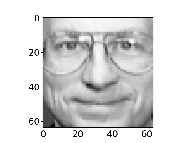
Figure: Data set from Olivetti Research Laboratory of faces.

Note that to display the face we had to reshape the appropriate row of the data matrix. This is because the images are turned into vectors by stacking columns of the image on top of each other to form a vector. The operation

im = np.reshape(Y[1, :].flatten(), (64, 64)).T

recovers the original image into a matrix im by using the np.reshape function to return the vector to a matrix.}

Visualizing the Eigenvectors

Each retained eigenvector is stored in the \(j\)th column of \(\mathbf{U}\). Each of these eigenvectors is associated with particular directions of variation in the original data. Principal component analysis implies that we can reconstruct any face by using a weighted sum of these eigenvectors where the weights for each face are given by the relevant vector of the latent variables, \(\mathbf{ z}_{i, :}\) and the diagonal elements of the matrix \(\mathbf{L}\). We can visualize the eigenvectors \(\mathbf{U}\) as images by performing the same reshape operation we used to recover the image associated with a data point above. Below we do this for the first nine eigenvectors of the Olivetti Faces data.

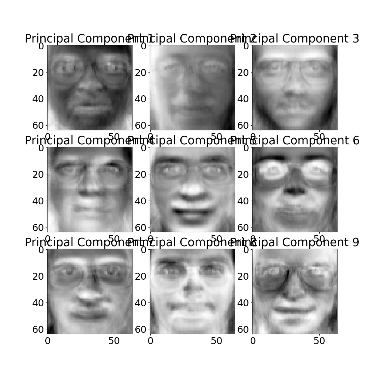
Figure: First 9 eigenvectors of the Olivetti faces data.

Reconstruction

We can now attempt to reconstruct a given training point from these eigenvectors. As we mentioned above, the reconstruction is dependent on the value of the latent variable and the weights from the matrix \(\mathbf{L}\). First let’s compute the value of the latent variables for the point we want to construct. Then we’ll use them to compute the weightings of each of the eigenvectors.

mu_x, C_x = posterior(Y, U, ell, sigma2)
reconstruction_weights = mu_x[display_index, :]*ell
print(reconstruction_weights)

This vector of reconstruction weights is applied to the ‘template images’ given by the eigenvectors to give us our reconstruction. Below we weight these templates and combine to form the reconstructed image, and show the comparison to the original image.

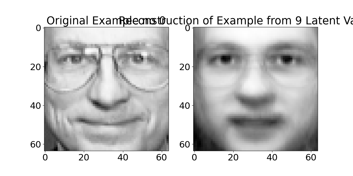
Figure: Reconstruction from the latent space of the faces data.

The quality of the reconstruction is a bit blurry, it can be improved by increasing the number of template images used (i.e. increasing the latent dimensionality).

Gene Expression

Each of the cells in your body stores your entire genetic code in your DNA, but at any one moment it is only ‘expressing’ a small portion of that code. Your cells are mainly constructed of protein, and these proteins are manufactured by first transcribing the DNA to RNA and then translating the RNA to protein. If the DNA is the cells hard drive, then one role of the RNA is to act like a cache of data that is being read from the hard drive at any one time. Gene expression arrays allow us to measure the quantity of different types of RNA in the cell, effectively analyzing what’s in the cache (although we have to destroy the cell or the tissue to access it). A gene expression experiment often consists of a time course or a series of experiments that characterise the gene expression of cells at any given time.

We will now load in one of the earliest gene expression data sets from a 1998 paper by Spellman et al., it consists of gene expression measurements of over six thousand genes in a range of conditions for brewer’s yeast. The experiment was designed for understanding the cell cycle of the genes. The expectation is that there should be oscillating signals inside the cell.

First we extract the principal components of the gene expression.

import pods

# load in data and replace missing values with zero
data=pods.datasets.spellman_yeast_cdc15()
Y = data['Y'].fillna(0)
q = 5
U, ell, sigma2 = ppca(Y, q)
mu_x, C_x = posterior(Y, U, ell, sigma2)

Now, looking through, we find that there is indeed a latent variable that appears to oscilate at approximately the right frequency. The 4th latent dimension (index=3) can be plotted across the time course as follows.

To reveal an oscillating shape. We can see which genes correspond to this shape by examining the associated column of \(\mathbf{U}\). Let’s augment our data matrix with this score.

gene_list = Y.T
gene_list['oscilation'] = np.sqrt(U[:, 3]**2)
gene_list.sort(columns='oscilation', ascending=False).index[:4]

We can look up the first three genes in this list which now ranks the genes according to how strongly they respond to the fourth latent dimension. The NCBI gene database allows us to search for the function of these genes. Looking at the function of the four genes that respond most strongly to the third latent variable they are all genes that encode histone proteins. The histone is thesupport scaffold for the DNA that ensures it folds correctly within the cell creating the nucleosomes. It seems to make sense that production of histone proteins should be strongly correlated with the cell cycle, as when the cell divides it needs to create a large number of histone proteins for creating the duplicated nucleosomes. The relevant links giving the descriptions of each gene given here: YDR224C, YDR225W, YBL003C and YNL030W.

Further Reading

• Chapter 7 up to pg 249 of Rogers and Girolami (2011)

Thanks!

For more information on these subjects and more you might want to check the following resources.

• twitter: @lawrennd
• podcast: The Talking Machines
• newspaper: Guardian Profile Page
• blog: http://inverseprobability.com

References