Visualisation

Review

• Last time: Looked at Generalised Linear Models.
• This time: visualisation with “unsupervised learning”

Clustering

Clustering

• One common approach, not deeply covered in this course.
• Associate each data point, \(\mathbf{ y}_{i, :}\) with one of \(k\) different discrete groups.
• For example:
  • Clustering animals into discrete groups. Are animals discrete or continuous?
  • Clustering into different different political affiliations.
• Humans do seem to like clusters:
  • Very useful when interacting with biologists.
• Subtle difference between clustering and vector quantisation

Trying to Teach About Infinity

• Little anecdote.

Clustering and Vector Quantisation

• To my mind difference is in clustering there should be a reduction in data density between samples.
• This definition is not universally applied.
• For today’s purposes we merge them:
  • Determine how to allocate each point to a group and harder total number of groups.

\(k\)-means Clustering

• Simple algorithm for allocating points to groups.
• Require: Set of \(k\) cluster centres & assignment of each points to a cluster.

1. Initialize cluster centres as randomly selected data points.
   2. Assign each data point to nearest cluster centre.
   3. Update each cluster centre by setting it to the mean of assigned data points.
   4. Repeat 2 and 3 until cluster allocations do not change.

Objective Function

• This minimizes the objective \[ E=\sum_{j=1}^K \sum_{i\ \text{allocated to}\ j} \left(\mathbf{ y}_{i, :} - \boldsymbol{ \mu}_{j, :}\right)^\top\left(\mathbf{ y}_{i, :} - \boldsymbol{ \mu}_{j, :}\right) \] i.e. it minimizes thesum of Euclidean squared distances betwen points and their associated centres.

• The minimum is not guaranteed to be global or unique.

• This objective is a non-convex optimization problem.

• Task: associate each data point with a different label.

• Label is not provided.

• Quite intuitive for humans, we do it naturally.

Platonic Ideals

• Names for animals originally invented by humans through ‘clustering’
• Can we have the computer to recreate that process of inventing the label?
• Greek philosopher, Plato, thought about ideas, he considered the concept of the Platonic ideal.
• Platonic ideal bird is the bird that is most bird-like or the chair that is most chair-like.

Cluster Center

• Can define different clusters, by finding their Platonic ideal (known as the cluster center)
• Allocate each data point to the relevant nearest cluster center.
• Allocate each animal to the class defined by its nearest cluster center.

Similarity and Distance Measures

• Define a notion of either similarity or distance between the objects and their Platonic ideal.
• If objects are vectors of data, \(\mathbf{ x}_i\).
• Represent cluster center for category \(j\) by a vector \(\boldsymbol{ \mu}_j\).
• This vector contains the ideal features of a bird, a chair, or whatever category \(j\) is.

Similarity or Distance

• Can either think in terms of similarity of the objects, or distances.
• We want objects that are similar to each other to cluster together. We want objects that are distant from each other to cluster apart.
• Use mathematical function to formalize this notion, e.g. for distance \[ d_{ij} = f(\mathbf{ x}_i, \boldsymbol{ \mu}_j). \]

Squared Distance

• Find cluster centers that are close to as many data points as possible.
• A commonly used distance is the squared distance, \[ d_{ij} = (\mathbf{ x}_i - \boldsymbol{ \mu}_j)^2. \]
• Already seen for regression.

Objective Function

• Given similarity measure, need number of cluster centers, \(K\).
• Find their location by allocating each center to a sub-set of the points and minimizing the sum of the squared errors, \[ E(\mathbf{M}) = \sum_{i \in \mathbf{i}_j} (\mathbf{ x}_i - \boldsymbol{ \mu}_j)^2 \] here \(\mathbf{i}_j\) is all indices of data points allocated to the \(j\)th center.

\(k\)-Means Clustering

• \(k\)-means clustering is simple and quick to implement.
• Very initialisation sensitive.

Initialisation

• Initialisation is the process of selecting a starting set of parameters.
• Optimisation result can depend on the starting point.
• For \(k\)-means clustering you need to choose an initial set of centers.
• Optimisation surface has many local optima, algorithm gets stuck in ones near initialisation.

\(k\)-Means Clustering

❮ ❯

Clustering with the \(k\)-means clustering algorithm.

\(k\)-Means Clustering

\(k\)-means clustering by Alex Ihler

Hierarchical Clustering

• Form taxonomies of the cluster centers
• Like humans apply to animals, to form phylogenies

Phylogenetic Trees

• Perform a hierarchical clustering based on genetic data, i.e. the actual contents of the genome.
• Perform across a number of species and produce a phylogenetic tree.
• Represents a guess at actual evolution of the species.
• Used to estimate the origin of viruses like AIDS or Bird flu

Product Clustering

• Could apply hierarchical clustering to an e-commerce company’s products.
• Would give us a phylogeny of products.
• Each cluster of products would be split into sub-clusters of products until we got down to individual products.
  • E.g. at high level Electronics/Clothing

Hierarchical Clustering Challenge

• Many products belong in more than one cluster: e.g. running shoes are ‘sporting goods’ and they are ‘clothing’.
• Tree structure doesn’t allow this allocation.
• Our own psychological grouping capabilities are in cognitive science.
  • E.g. Josh Tenenbaum and collaborators cluster data in more complex ways.

Other Clustering Approaches

• Spectral clustering (Shi and Malik (2000),Ng et al. (n.d.))
  • Allows clusters which aren’t convex hulls.
• Dirichlet process
  • A probabilistic formulation for a clustering algorithm that is non-parametric.
  • Loosely speaking it allows infinite clusters
  • In practice useful for dealing with previously unknown species (e.g. a “Black Swan Event”).

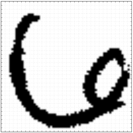
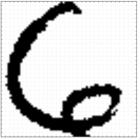
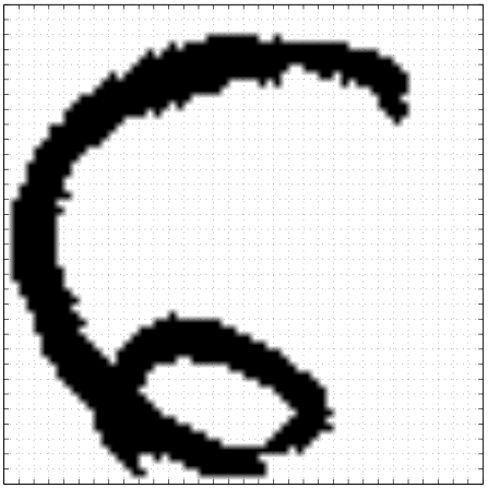
High Dimensional Data

• USPS Data Set Handwritten Digit
• 3648 dimensions (64 rows, 57 columns)
• Space contains much more than just this digit.

USPS Samples

❮ ❯

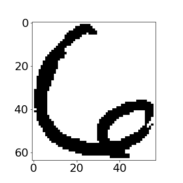
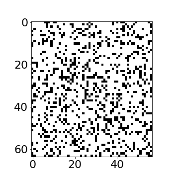
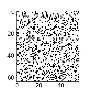
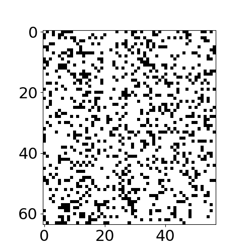
• Even if we sample every nanonsecond from now until end of universe you won’t see original six!

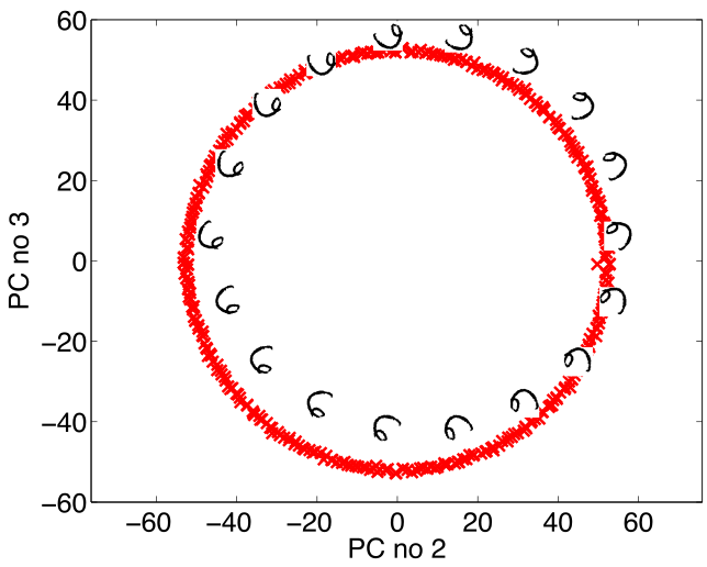
Simple Model of Digit

• Rotate a prototype

❮ ❯

Low Dimensional Manifolds

• Pure rotation is too simple
  • In practice data may undergo several distortions.
• For high dimensional data with structure:
  • We expect fewer distortions than dimensions;
  • Therefore we expect the data to live on a lower dimensional manifold.
  • Conclusion: Deal with high dimensional data by looking for a lower dimensional non-linear embedding.

Latent Variables

Your Personality

Factor Analysis Model

\[ \mathbf{ y}= \mathbf{f}(\mathbf{ z}) + \boldsymbol{ \epsilon}, \]

\[ \mathbf{f}(\mathbf{ z}) = \mathbf{W}\mathbf{ z} \]

Closely Related to Linear Regression

\[ \mathbf{f}(\mathbf{ z}) = \begin{bmatrix} f_1(\mathbf{ z}) \\ f_2(\mathbf{ z}) \\ \vdots \\ f_p(\mathbf{ z})\end{bmatrix} \]

\[ f_j(\mathbf{ z}) = \mathbf{ w}_{j, :}^\top \mathbf{ z}, \]

\[ \epsilon_j \sim \mathcal{N}\left(0,\sigma^2_j\right). \]

Data Representation

\[ \mathbf{Y} = \begin{bmatrix} \mathbf{ y}_{1, :}^\top \\ \mathbf{ y}_{2, :}^\top \\ \vdots \\ \mathbf{ y}_{n, :}^\top\end{bmatrix}, \]

\[ \mathbf{F} = \mathbf{Z}\mathbf{W}^\top, \]

Latent Variables vs Linear Regression

\[ x_{i,j} \sim \mathcal{N}\left(0,1\right), \] and we can write the density governing the latent variable associated with a single point as, \[ \mathbf{ z}_{i, :} \sim \mathcal{N}\left(\mathbf{0},\mathbf{I}\right). \]

\[ \mathbf{f}_{i, :} = \mathbf{f}(\mathbf{ z}_{i, :}) = \mathbf{W}\mathbf{ z}_{i, :} \]

\[ \mathbf{f}_{i, :} \sim \mathcal{N}\left(\mathbf{0},\mathbf{W}\mathbf{W}^\top\right) \]

Data Distribution

\[ \mathbf{ y}_{i, :} = \sim \mathcal{N}\left(\mathbf{0},\mathbf{W}\mathbf{W}^\top + \boldsymbol{\Sigma}\right) \]

\[ \boldsymbol{\Sigma} = \begin{bmatrix}\sigma^2_{1} & 0 & 0 & 0\\ 0 & \sigma^2_{2} & 0 & 0\\ 0 & 0 & \ddots & 0\\ 0 & 0 & 0 & \sigma^2_p\end{bmatrix}. \]

Mean Vector

\[ \mathbf{ y}_{i, :} = \mathbf{W}\mathbf{ z}_{i, :} + \boldsymbol{ \mu}+ \boldsymbol{ \epsilon}_{i, :} \]

\[ \boldsymbol{ \mu}= \frac{1}{n} \sum_{i=1}^n \mathbf{ y}_{i, :}, \] \(\mathbf{C}= \mathbf{W}\mathbf{W}^\top + \boldsymbol{\Sigma}\)

Principal Component Analysis

Hotelling (1933) took \(\sigma^2_i \rightarrow 0\) so \[ \mathbf{ y}_{i, :} \sim \lim_{\sigma^2 \rightarrow 0} \mathcal{N}\left(\mathbf{0},\mathbf{W}\mathbf{W}^\top + \sigma^2 \mathbf{I}\right). \]

Degenerate Covariance

\[ p(\mathbf{ y}_{i, :}|\mathbf{W}) = \lim_{\sigma^2 \rightarrow 0} \frac{1}{(2\pi)^\frac{p}{2} |\mathbf{W}\mathbf{W}^\top + \sigma^2 \mathbf{I}|^{\frac{1}{2}}} \exp\left(-\frac{1}{2}\mathbf{ y}_{i, :}\left[\mathbf{W}\mathbf{W}^\top+ \sigma^2 \mathbf{I}\right]^{-1}\mathbf{ y}_{i, :}\right), \]

Computation of the Marginal Likelihood

\[ \mathbf{ y}_{i,:}=\mathbf{W}\mathbf{ z}_{i,:}+\boldsymbol{ \epsilon}_{i,:},\quad \mathbf{ z}_{i,:} \sim \mathcal{N}\left(\mathbf{0},\mathbf{I}\right), \quad \boldsymbol{ \epsilon}_{i,:} \sim \mathcal{N}\left(\mathbf{0},\sigma^{2}\mathbf{I}\right) \]

\[ \mathbf{W}\mathbf{ z}_{i,:} \sim \mathcal{N}\left(\mathbf{0},\mathbf{W}\mathbf{W}^\top\right) \]

\[ \mathbf{W}\mathbf{ z}_{i, :} + \boldsymbol{ \epsilon}_{i, :} \sim \mathcal{N}\left(\mathbf{0},\mathbf{W}\mathbf{W}^\top + \sigma^2 \mathbf{I}\right) \]

Linear Latent Variable Model II

Probabilistic PCA Max. Likelihood Soln (Tipping and Bishop (1999))

\[p\left(\mathbf{Y}|\mathbf{W}\right)=\prod_{i=1}^{n}\mathcal{N}\left(\mathbf{ y}_{i, :}|\mathbf{0},\mathbf{W}\mathbf{W}^{\top}+\sigma^{2}\mathbf{I}\right)\]

Linear Latent Variable Model II

Probabilistic PCA Max. Likelihood Soln (Tipping and Bishop (1999)) \[ p\left(\mathbf{Y}|\mathbf{W}\right)=\prod_{i=1}^{n}\mathcal{N}\left(\mathbf{ y}_{i,:}|\mathbf{0},\mathbf{C}\right),\quad \mathbf{C}=\mathbf{W}\mathbf{W}^{\top}+\sigma^{2}\mathbf{I} \] \[ \log p\left(\mathbf{Y}|\mathbf{W}\right)=-\frac{n}{2}\log\left|\mathbf{C}\right|-\frac{1}{2}\text{tr}\left(\mathbf{C}^{-1}\mathbf{Y}^{\top}\mathbf{Y}\right)+\text{const.} \] If \(\mathbf{U}_{q}\) are first \(q\) principal eigenvectors of \(n^{-1}\mathbf{Y}^{\top}\mathbf{Y}\) and the corresponding eigenvalues are \(\boldsymbol{\Lambda}_{q}\), \[ \mathbf{W}=\mathbf{U}_{q}\mathbf{L}\mathbf{R}^{\top},\quad\mathbf{L}=\left(\boldsymbol{\Lambda}_{q}-\sigma^{2}\mathbf{I}\right)^{\frac{1}{2}} \] where \(\mathbf{R}\) is an arbitrary rotation matrix.

Principal Component Analysis

• PCA (Hotelling (1933)) is a linear embedding.
• Today its presented as:
  • Rotate to find ‘directions’ in data with maximal variance.
  • How do we find these directions?
• Algorithmically we do this by diagonalizing the sample covariance matrix \[ \mathbf{S}=\frac{1}{n}\sum_{i=1}^n\left(\mathbf{ y}_{i, :}-\boldsymbol{ \mu}\right)\left(\mathbf{ y}_{i, :} - \boldsymbol{ \mu}\right)^\top \]

Principal Component Analysis

• Find directions in the data, \(\mathbf{ z}= \mathbf{U}\mathbf{ y}\), for which variance is maximized.

Lagrangian

• Solution is found via constrained optimisation (which uses Lagrange multipliers): \[ L\left(\mathbf{u}_{1},\lambda_{1}\right)=\mathbf{u}_{1}^{\top}\mathbf{S}\mathbf{u}_{1}+\lambda_{1}\left(1-\mathbf{u}_{1}^{\top}\mathbf{u}_{1}\right) \]

• Gradient with respect to \(\mathbf{u}_{1}\) \[\frac{\text{d}L\left(\mathbf{u}_{1},\lambda_{1}\right)}{\text{d}\mathbf{u}_{1}}=2\mathbf{S}\mathbf{u}_{1}-2\lambda_{1}\mathbf{u}_{1}\] rearrange to form \[\mathbf{S}\mathbf{u}_{1}=\lambda_{1}\mathbf{u}_{1}.\] Which is known as an eigenvalue problem.

• Further directions that are orthogonal to the first can also be shown to be eigenvectors of the covariance.

Linear Dimensionality Reduction

• Represent data, \(\mathbf{Y}\), with a lower dimensional set of latent variables \(\mathbf{Z}\).
• Assume a linear relationship of the form \[ \mathbf{ y}_{i,:}=\mathbf{W}\mathbf{ z}_{i,:}+\boldsymbol{ \epsilon}_{i,:}, \] where \[ \boldsymbol{ \epsilon}_{i,:} \sim \mathcal{N}\left(\mathbf{0},\sigma^2\mathbf{I}\right) \]

Linear Latent Variable Model

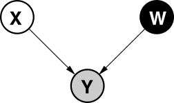
Probabilistic PCA

Define linear-Gaussian relationship between latent variables and data. Standard Latent variable approach: Define Gaussian prior over latent space, \(\mathbf{Z}\). Integrate out latent variables.

\[ p\left(\mathbf{Y}|\mathbf{Z},\mathbf{W}\right)=\prod_{i=1}^{n}\mathcal{N}\left(\mathbf{ y}_{i,:}|\mathbf{W}\mathbf{ z}_{i,:},\sigma^2\mathbf{I}\right) \] \[ p\left(\mathbf{Z}\right)=\prod_{i=1}^{n}\mathcal{N}\left(\mathbf{ z}_{i,:}|\mathbf{0},\mathbf{I}\right) \] \[ p\left(\mathbf{Y}|\mathbf{W}\right)=\prod_{i=1}^{n}\mathcal{N}\left(\mathbf{ y}_{i,:}|\mathbf{0},\mathbf{W}\mathbf{W}^{\top}+\sigma^{2}\mathbf{I}\right) \]

Examples: Motion Capture Data

Robot Navigation Example

• Example involving 215 observations of 30 access points.
• Infer location of ‘robot’ and accesspoints.
• This is known as SLAM (simulataneous localization and mapping).

Interpretations of Principal Component Analysis

Relationship to Matrix Factorization

• PCA is closely related to matrix factorisation.

• Instead of \(\mathbf{Z}\), \(\mathbf{W}\)

• Define Users \(\mathbf{U}\) and items \(\mathbf{V}\)

• Matrix factorisation: \[ f_{i, j} = \mathbf{u}_{i, :}^\top \mathbf{v}_{j, :} \] PCA: \[ f_{i, j} = \mathbf{ z}_{i, :}^\top \mathbf{ w}_{j, :} \]

Other Interpretations of PCA: Separating Model and Algorithm

• PCA introduced as latent variable model (a model).
• Solution is through an eigenvalue problem (an algorithm).
• This causes some confusion about what PCA is.

\[ \mathbf{Y}= \mathbf{V} \boldsymbol{\Lambda} \mathbf{U}^\top \]

\[ \mathbf{Y}^\top\mathbf{Y}= \mathbf{U}\boldsymbol{\Lambda}\mathbf{V}^\top\mathbf{V} \boldsymbol{\Lambda} \mathbf{U}^\top = \mathbf{U}\boldsymbol{\Lambda}^2 \mathbf{U}^\top \]

Separating Model and Algorithm

• Separation between model and algorithm is helpful conceptually.
• Even if in practice they conflate (e.g. deep neural networks).
• Sometimes difficult to pull apart.
• Helpful to revisit algorithms with modelling perspective in mind.
  • Probabilistic numerics

PPCA Marginal Likelihood

We have developed the posterior density over the latent variables given the data and the parameters, and due to symmetries in the underlying prediction function, it has a very similar form to its sister density, the posterior of the weights given the data from Bayesian regression. Two key differences are as follows. If we were to do a Bayesian multiple output regression we would find that the marginal likelihood of the data is independent across the features and correlated across the data, \[ p(\mathbf{Y}|\mathbf{Z}) = \prod_{j=1}^p \mathcal{N}\left(\mathbf{ y}_{:, j}|\mathbf{0}, \alpha\mathbf{Z}\mathbf{Z}^\top + \sigma^2 \mathbf{I}\right) \] where \(\mathbf{ y}_{:, j}\) is a column of the data matrix and the independence is across the features, in probabilistic PCA the marginal likelihood has the form, \[ p(\mathbf{Y}|\mathbf{W}) = \prod_{i=1}^n\mathcal{N}\left(\mathbf{ y}_{i, :}|\mathbf{0},\mathbf{W}\mathbf{W}^\top + \sigma^2 \mathbf{I}\right) \] where \(\mathbf{ y}_{i, :}\) is a row of the data matrix \(\mathbf{Y}\) and the independence is across the data points.

Computation of the Log Likelihood

The quality of the model can be assessed using the log likelihood of this Gaussian form. \[ \log p(\mathbf{Y}|\mathbf{W}) = -\frac{n}{2} \log \left| \mathbf{W}\mathbf{W}^\top + \sigma^2 \mathbf{I}\right| -\frac{1}{2} \sum_{i=1}^n\mathbf{ y}_{i, :}^\top \left(\mathbf{W}\mathbf{W}^\top + \sigma^2 \mathbf{I}\right)^{-1} \mathbf{ y}_{i, :} +\text{const} \] but this can be computed more rapidly by exploiting the low rank form of the covariance covariance, \(\mathbf{C}= \mathbf{W}\mathbf{W}^\top + \sigma^2 \mathbf{I}\) and the fact that \(\mathbf{W}= \mathbf{U}\mathbf{L}\mathbf{R}^\top\). Specifically, we first use the decomposition of \(\mathbf{W}\) to write: \[ -\frac{n}{2} \log \left| \mathbf{W}\mathbf{W}^\top + \sigma^2 \mathbf{I}\right| = -\frac{n}{2} \sum_{i=1}^q \log (\ell_i^2 + \sigma^2) - \frac{n(p-q)}{2}\log \sigma^2, \] where \(\ell_i\) is the \(i\)th diagonal element of \(\mathbf{L}\). Next, we use the Woodbury matrix identity which allows us to write the inverse as a quantity which contains another inverse in a smaller matrix: \[ (\sigma^2 \mathbf{I}+ \mathbf{W}\mathbf{W}^\top)^{-1} = \sigma^{-2}\mathbf{I}-\sigma^{-4}\mathbf{W}{\underbrace{(\mathbf{I}+\sigma^{-2}\mathbf{W}^\top\mathbf{W})}_{\mathbf{C}_x}}^{-1}\mathbf{W}^\top \] So, it turns out that the original inversion of the \(p \times p\) matrix can be done by forming a quantity which contains the inversion of a \(q \times q\) matrix which, moreover, turns out to be the quantity \(\mathbf{C}_x\) of the posterior.

Now, we put everything together to obtain: \[ \log p(\mathbf{Y}|\mathbf{W}) = -\frac{n}{2} \sum_{i=1}^q \log (\ell_i^2 + \sigma^2) - \frac{n(p-q)}{2}\log \sigma^2 - \frac{1}{2} \text{tr}\left(\mathbf{Y}^\top \left( \sigma^{-2}\mathbf{I}-\sigma^{-4}\mathbf{W}\mathbf{C}_x \mathbf{W}^\top \right) \mathbf{Y}\right) + \text{const}, \] where we used the fact that a scalar sum can be written as \(\sum_{i=1}^n\mathbf{ y}_{i,:}^\top \mathbf{K}\mathbf{ y}_{i,:} = \text{tr}\left(\mathbf{Y}^\top \mathbf{K}\mathbf{Y}\right)\), for any matrix \(\mathbf{K}\) of appropriate dimensions. We now use the properties of the trace \(\text{tr}\left(\mathbf{A}+\mathbf{B}\right)=\text{tr}\left(\mathbf{A}\right)+\text{tr}\left(\mathbf{B}\right)\) and \(\text{tr}\left(c \mathbf{A}\right) = c \text{tr}\left(\mathbf{A}\right)\), where \(c\) is a scalar and \(\mathbf{A},\mathbf{B}\) matrices of compatible sizes. Therefore, the final log likelihood takes the form: \[ \log p(\mathbf{Y}|\mathbf{W}) = -\frac{n}{2} \sum_{i=1}^q \log (\ell_i^2 + \sigma^2) - \frac{n(p-q)}{2}\log \sigma^2 - \frac{\sigma^{-2}}{2} \text{tr}\left(\mathbf{Y}^\top \mathbf{Y}\right) +\frac{\sigma^{-4}}{2} \text{tr}\left(\mathbf{B}\mathbf{C}_x\mathbf{B}^\top\right) + \text{const} \] where we also defined \(\mathbf{B}=\mathbf{Y}^\top\mathbf{W}\). Finally, notice that \(\text{tr}\left(\mathbf{Y}\mathbf{Y}^\top\right)=\text{tr}\left(\mathbf{Y}^\top\mathbf{Y}\right)\) can be computed faster as the sum of all the elements of \(\mathbf{Y}\circ\mathbf{Y}\), where \(\circ\) denotes the element-wise (or Hadamard) product.

Reconstruction of the Data

Given any posterior projection of a data point, we can replot the original data as a function of the input space.

We will now try to reconstruct the motion capture figure form some different places in the latent plot.

Other Data Sets to Explore

Below there are a few other data sets from pods you might want to explore with PCA. Both of them have \(p\)>\(n\) so you need to consider how to do the larger eigenvalue probleme efficiently without large demands on computer memory.

The data is actually quite high dimensional, and solving the eigenvalue problem in the high dimensional space can take some time. At this point we turn to a neat trick, you don’t have to solve the full eigenvalue problem in the \(p\times p\) covariance, you can choose instead to solve the related eigenvalue problem in the \(n\times n\) space, and in this case \(n=200\) which is much smaller than \(p\).

The original eigenvalue problem has the form \[ \mathbf{Y}^\top\mathbf{Y}\mathbf{U} = \mathbf{U}\boldsymbol{\Lambda} \] But if we premultiply by \(\mathbf{Y}\) then we can solve, \[ \mathbf{Y}\mathbf{Y}^\top\mathbf{Y}\mathbf{U} = \mathbf{Y}\mathbf{U}\boldsymbol{\Lambda} \] but it turns out that we can write \[ \mathbf{U}^\prime = \mathbf{Y}\mathbf{U} \Lambda^{\frac{1}{2}} \] where \(\mathbf{U}^\prime\) is an orthorormal matrix because \[ \left.\mathbf{U}^\prime\right.^\top\mathbf{U}^\prime = \Lambda^{-\frac{1}{2}}\mathbf{U}\mathbf{Y}^\top\mathbf{Y}\mathbf{U} \Lambda^{-\frac{1}{2}} \] and since \(\mathbf{U}\) diagonalises \(\mathbf{Y}^\top\mathbf{Y}\), \[ \mathbf{U}\mathbf{Y}^\top\mathbf{Y}\mathbf{U} = \Lambda \] then \[ \left.\mathbf{U}^\prime\right.^\top\mathbf{U}^\prime = \mathbf{I} \]

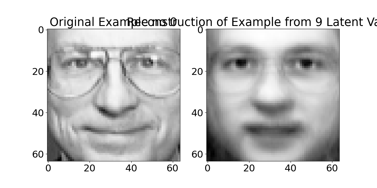
Olivetti Faces

```

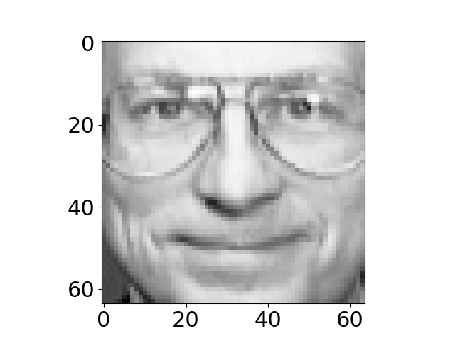
recovers the original image into a matrix im by using the np.reshape function to return the vector to a matrix.}

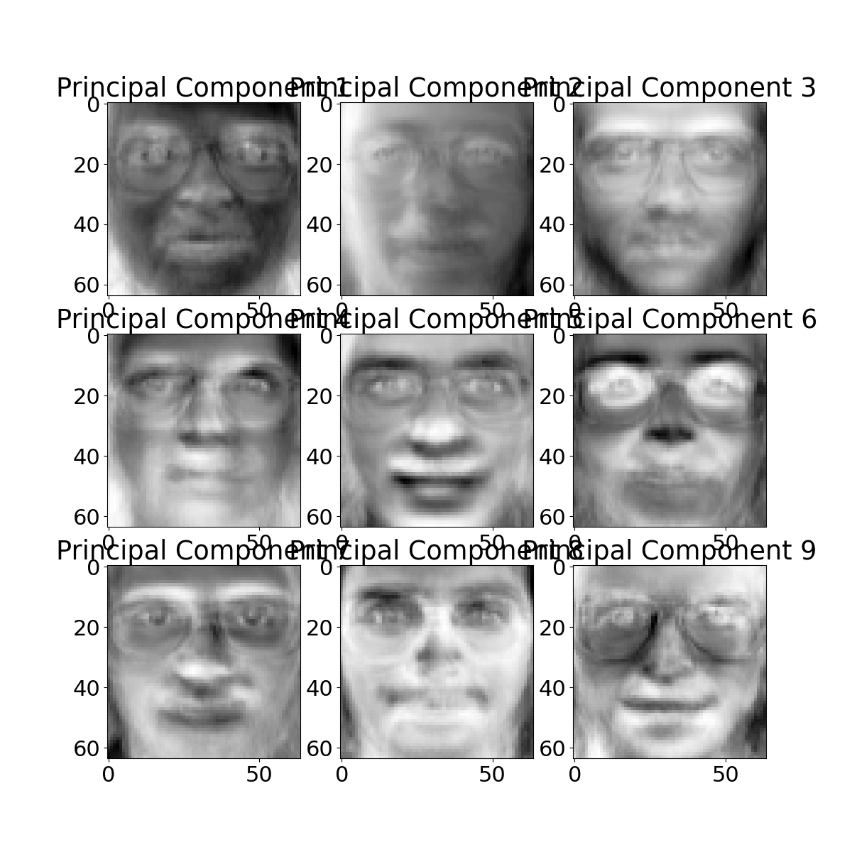
Visualizing the Eigenvectors

Reconstruction

Gene Expression

Each of the cells in your body stores your entire genetic code in your DNA, but at any one moment it is only ‘expressing’ a small portion of that code. Your cells are mainly constructed of protein, and these proteins are manufactured by first transcribing the DNA to RNA and then translating the RNA to protein. If the DNA is the cells hard drive, then one role of the RNA is to act like a cache of data that is being read from the hard drive at any one time. Gene expression arrays allow us to measure the quantity of different types of RNA in the cell, effectively analyzing what’s in the cache (although we have to destroy the cell or the tissue to access it). A gene expression experiment often consists of a time course or a series of experiments that characterise the gene expression of cells at any given time.

We will now load in one of the earliest gene expression data sets from a 1998 paper by Spellman et al., it consists of gene expression measurements of over six thousand genes in a range of conditions for brewer’s yeast. The experiment was designed for understanding the cell cycle of the genes. The expectation is that there should be oscillating signals inside the cell.

First we extract the principal components of the gene expression.

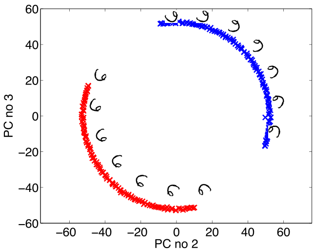
Now, looking through, we find that there is indeed a latent variable that appears to oscilate at approximately the right frequency. The 4th latent dimension (index=3) can be plotted across the time course as follows.

To reveal an oscillating shape. We can see which genes correspond to this shape by examining the associated column of \(\mathbf{U}\). Let’s augment our data matrix with this score.