R250: Gaussian Processes Introduction

Laplace’s Gremlin

What is Machine Learning?

What is Machine Learning?

What is Machine Learning?

\[\text{data} + \text{model} \stackrel{\text{compute}}{\rightarrow} \text{prediction}\]

• To combine data with a model need:
• a prediction function \(f(\cdot)\) includes our beliefs about the regularities of the universe
• an objective function \(E(\cdot)\) defines the cost of misprediction.

Artificial Intelligence

• Machine learning is a mainstay because of importance of prediction.

Uncertainty

• Uncertainty in prediction arises from:
• scarcity of training data and
• mismatch between the set of prediction functions we choose and all possible prediction functions.
• Also uncertainties in objective, leave those for another day.

Neural Networks and Prediction Functions

• adaptive non-linear function models inspired by simple neuron models (McCulloch and Pitts, 1943)
• have become popular because of their ability to model data.
• can be composed to form highly complex functions
• start by focussing on one hidden layer

Prediction Function of One Hidden Layer

\[ f(\mathbf{ x}) = \left.\mathbf{ w}^{(2)}\right.^\top \boldsymbol{ \phi}(\mathbf{W}_{1}, \mathbf{ x}) \]

\(f(\cdot)\) is a scalar function with vector inputs,

\(\boldsymbol{ \phi}(\cdot)\) is a vector function with vector inputs.

• dimensionality of the vector function is known as the number of hidden units, or the number of neurons.

• elements of \(\boldsymbol{ \phi}(\cdot)\) are the activation function of the neural network

• elements of \(\mathbf{W}_{1}\) are the parameters of the activation functions.

Relations with Classical Statistics

• In statistics activation functions are known as basis functions.

• would think of this as a linear model: not linear predictions, linear in the parameters

• \(\mathbf{ w}_{1}\) are static parameters.

Adaptive Basis Functions

• In machine learning we optimize \(\mathbf{W}_{1}\) as well as \(\mathbf{W}_{2}\) (which would normally be denoted in statistics by \(\boldsymbol{\beta}\)).

Integrated Basis Functions

• Revisit that decision: follow the path of Neal (1994) and MacKay (1992).

• Consider the probabilistic approach.

Probabilistic Modelling

• Probabilistically we want, \[ p(y_*|\mathbf{ y}, \mathbf{X}, \mathbf{ x}_*), \] \(y_*\) is a test output \(\mathbf{ x}_*\) is a test input \(\mathbf{X}\) is a training input matrix \(\mathbf{ y}\) is training outputs

Joint Model of World

\[ p(y_*|\mathbf{ y}, \mathbf{X}, \mathbf{ x}_*) = \int p(y_*|\mathbf{ x}_*, \mathbf{W}) p(\mathbf{W}| \mathbf{ y}, \mathbf{X}) \text{d} \mathbf{W} \]

Likelihood

\(p(y|\mathbf{ x}, \mathbf{W})\) is the likelihood of data point

Likelihood and Prediction Function

\[ p(y_i | f(\mathbf{ x}_i)) = \frac{1}{\sqrt{2\pi \sigma^2}} \exp\left(-\frac{\left(y_i - f(\mathbf{ x}_i)\right)^2}{2\sigma^2}\right) \]

Unsupervised Learning

• Can also consider priors over latents \[ p(\mathbf{ y}_*|\mathbf{ y}) = \int p(\mathbf{ y}_*|\mathbf{X}_*, \mathbf{W}) p(\mathbf{W}| \mathbf{ y}, \mathbf{X}) p(\mathbf{X}) p(\mathbf{X}_*) \text{d} \mathbf{W}\text{d} \mathbf{X}\text{d}\mathbf{X}_* \]

• This gives unsupervised learning.

Probabilistic Inference

• Data: \(\mathbf{ y}\)

• Model: \(p(\mathbf{ y}, \mathbf{ y}^*)\)

• Prediction: \(p(\mathbf{ y}^*| \mathbf{ y})\)

Graphical Models

• Represent joint distribution through conditional dependencies.
• E.g. Markov chain

\[p(\mathbf{ y}) = p(y_n| y_{n-1}) p(y_{n-1}|y_{n-2}) \dots p(y_{2} | y_{1})\]

Predict Perioperative Risk of Clostridium Difficile Infection Following Colon Surgery (Steele et al., 2012)

Performing Inference

• Easy to write in probabilities

• But underlying this is a wealth of computational challenges.

• High dimensional integrals typically require approximation.

Linear Models

• In statistics, focussed more on linear model implied by \[ f(\mathbf{ x}) = \left.\mathbf{ w}^{(2)}\right.^\top \boldsymbol{ \phi}(\mathbf{W}_1, \mathbf{ x}) \]

• Hold \(\mathbf{W}_1\) fixed for given analysis.

• Gaussian prior for \(\mathbf{W}\), \[ \mathbf{ w}^{(2)} \sim \mathcal{N}\left(\mathbf{0},\mathbf{C}\right). \] \[ y_i = f(\mathbf{ x}_i) + \epsilon_i, \] where \[ \epsilon_i \sim \mathcal{N}\left(0,\sigma^2\right) \]

Linear Gaussian Models

• Normally integrals are complex but for this Gaussian linear case they are trivial.

Multivariate Gaussian Properties

Recall Univariate Gaussian Properties

Recall Univariate Gaussian Properties

2. Scaling a Gaussian leads to a Gaussian.

Multivariate Consequence

\[\mathbf{ x}\sim \mathcal{N}\left(\boldsymbol{ \mu},\mathbf{C}\right)\]

Linear Gaussian Models

1. linear Gaussian models are easier to deal with
2. Even the parameters within the process can be handled, by considering a particular limit.

Multivariate Gaussian Properties

• If \[ \mathbf{ y}= \mathbf{W}\mathbf{ x}+ \boldsymbol{ \epsilon}, \]

• Assume \[ \begin{align} \mathbf{ x}& \sim \mathcal{N}\left(\boldsymbol{ \mu},\mathbf{C}\right)\\ \boldsymbol{ \epsilon}& \sim \mathcal{N}\left(\mathbf{0},\boldsymbol{ \Sigma}\right) \end{align} \]

• Then \[ \mathbf{ y}\sim \mathcal{N}\left(\mathbf{W}\boldsymbol{ \mu},\mathbf{W}\mathbf{C}\mathbf{W}^\top + \boldsymbol{ \Sigma}\right). \] If \(\boldsymbol{ \Sigma}=\sigma^2\mathbf{I}\), this is Probabilistic PCA (Tipping and Bishop, 1999).

Linear Model Overview

• Set each activation function computed at each data point to be

\[ \phi_{i,j} = \phi(\mathbf{ w}^{(1)}_{j}, \mathbf{ x}_{i}) \] Define design matrix \[ \boldsymbol{ \Phi}= \begin{bmatrix} \phi_{1, 1} & \phi_{1, 2} & \dots & \phi_{1, h} \\ \phi_{1, 2} & \phi_{1, 2} & \dots & \phi_{1, n} \\ \vdots & \vdots & \ddots & \vdots \\ \phi_{n, 1} & \phi_{n, 2} & \dots & \phi_{n, h} \end{bmatrix}. \]

Matrix Representation of a Neural Network

\[y\left(\mathbf{ x}\right) = \boldsymbol{ \phi}\left(\mathbf{ x}\right)^\top \mathbf{ w}+ \epsilon\]

Multivariate Gaussian Properties

• If \[ \mathbf{ y}= \mathbf{W}\mathbf{ x}+ \boldsymbol{ \epsilon}, \]

• Assume \[ \begin{align} \mathbf{ x}& \sim \mathcal{N}\left(\boldsymbol{ \mu},\mathbf{C}\right)\\ \boldsymbol{ \epsilon}& \sim \mathcal{N}\left(\mathbf{0},\boldsymbol{ \Sigma}\right) \end{align} \]

• Then \[ \mathbf{ y}\sim \mathcal{N}\left(\mathbf{W}\boldsymbol{ \mu},\mathbf{W}\mathbf{C}\mathbf{W}^\top + \boldsymbol{ \Sigma}\right). \] If \(\boldsymbol{ \Sigma}=\sigma^2\mathbf{I}\), this is Probabilistic PCA (Tipping and Bishop, 1999).

Prior Density

• Define \[ \mathbf{ w}\sim \mathcal{N}\left(\mathbf{0},\alpha\mathbf{I}\right), \]
• Rules of multivariate Gaussians to see that, \[ \mathbf{ y}\sim \mathcal{N}\left(\mathbf{0},\alpha \boldsymbol{ \Phi}\boldsymbol{ \Phi}^\top + \sigma^2 \mathbf{I}\right). \]

\[ \mathbf{K}= \alpha \boldsymbol{ \Phi}\boldsymbol{ \Phi}^\top + \sigma^2 \mathbf{I}. \]

Joint Gaussian Density

• Elements are a function \(k_{i,j} = k\left(\mathbf{ x}_i, \mathbf{ x}_j\right)\)

\[ \mathbf{K}= \alpha \boldsymbol{ \Phi}\boldsymbol{ \Phi}^\top + \sigma^2 \mathbf{I}. \]

Covariance Function

\[ k_f\left(\mathbf{ x}_i, \mathbf{ x}_j\right) = \alpha \boldsymbol{ \phi}\left(\mathbf{W}_1, \mathbf{ x}_i\right)^\top \boldsymbol{ \phi}\left(\mathbf{W}_1, \mathbf{ x}_j\right) \]

• formed by inner products of the rows of the design matrix.

Gaussian Process

• Instead of making assumptions about our density over each data point, \(y_i\) as i.i.d.

• make a joint Gaussian assumption over our data.

• covariance matrix is now a function of both the parameters of the activation function, \(\mathbf{W}_1\), and the input variables, \(\mathbf{X}\).

• Arises from integrating out \(\mathbf{ w}^{(2)}\).

Basis Functions

• Can be very complex, such as deep kernels, (Cho and Saul, 2009) or could even put a convolutional neural network inside.
• Viewing a neural network in this way is also what allows us to beform sensible batch normalizations (Ioffe and Szegedy, 2015).

Non-degenerate Gaussian Processes

• This process is degenerate.
• Covariance function is of rank at most \(h\).
• As \(n\rightarrow \infty\), covariance matrix is not full rank.
• Leading to \(\det{\mathbf{K}} = 0\)

Infinite Networks

• In ML Radford Neal (Neal, 1994) asked “what would happen if you took \(h\rightarrow \infty\)?”

Roughly Speaking

• Instead of \[ \begin{align*} k_f\left(\mathbf{ x}_i, \mathbf{ x}_j\right) & = \alpha \boldsymbol{ \phi}\left(\mathbf{W}_1, \mathbf{ x}_i\right)^\top \boldsymbol{ \phi}\left(\mathbf{W}_1, \mathbf{ x}_j\right)\\ & = \alpha \sum_k \phi\left(\mathbf{ w}^{(1)}_k, \mathbf{ x}_i\right) \phi\left(\mathbf{ w}^{(1)}_k, \mathbf{ x}_j\right) \end{align*} \]
• Sample infinitely many from a prior density, \(p(\mathbf{ w}^{(1)})\), \[ k_f\left(\mathbf{ x}_i, \mathbf{ x}_j\right) = \alpha \int \phi\left(\mathbf{ w}^{(1)}, \mathbf{ x}_i\right) \phi\left(\mathbf{ w}^{(1)}, \mathbf{ x}_j\right) p(\mathbf{ w}^{(1)}) \text{d}\mathbf{ w}^{(1)} \]
• Also applies for non-Gaussian \(p(\mathbf{ w}^{(1)})\) because of the central limit theorem.

Simple Probabilistic Program

• If \[ \begin{align*} \mathbf{ w}^{(1)} & \sim p(\cdot)\\ \phi_i & = \phi\left(\mathbf{ w}^{(1)}, \mathbf{ x}_i\right), \end{align*} \] has finite variance.

• Then taking number of hidden units to infinity, is also a Gaussian process.

Further Reading

• Chapter 2 of Neal’s thesis (Neal, 1994)

• Rest of Neal’s thesis. (Neal, 1994)

• David MacKay’s PhD thesis (MacKay, 1992)

Distributions over Functions

Sampling a Function

Multi-variate Gaussians

• We will consider a Gaussian with a particular structure of covariance matrix.
• Generate a single sample from this 25 dimensional Gaussian density, \[ \mathbf{ f}=\left[f_{1},f_{2}\dots f_{25}\right]. \]
• We will plot these points against their index.

Gaussian Distribution Sample

❮ ❯

Sampling a Function from a Gaussian

❮ ❯

Joint Density of \(f_1\) and \(f_2\)

Prediction of \(f_{2}\) from \(f_{1}\)

❮ ❯

Uluru

Prediction with Correlated Gaussians

• Prediction of \(f_2\) from \(f_1\) requires conditional density.
• Conditional density is also Gaussian. \[ p(f_2|f_1) = \mathcal{N}\left(f_2|\frac{k_{1, 2}}{k_{1, 1}}f_1, k_{2, 2} - \frac{k_{1,2}^2}{k_{1,1}}\right) \] where covariance of joint density is given by \[ \mathbf{K}= \begin{bmatrix} k_{1, 1} & k_{1, 2}\\ k_{2, 1} & k_{2, 2}.\end{bmatrix} \]

Joint Density of \(f_1\) and \(f_8\)

Prediction of \(f_{8}\) from \(f_{1}\)

❮ ❯

Details

• The single contour of the Gaussian density represents the joint distribution, \(p(f_1, f_8)\)

Prediction with Correlated Gaussians

• Prediction of \(\mathbf{ f}_*\) from \(\mathbf{ f}\) requires multivariate conditional density.

• Multivariate conditional density is also Gaussian. \[ p(\mathbf{ f}_*|\mathbf{ f}) = {\mathcal{N}\left(\mathbf{ f}_*|\mathbf{K}_{*,\mathbf{ f}}\mathbf{K}_{\mathbf{ f},\mathbf{ f}}^{-1}\mathbf{ f},\mathbf{K}_{*,*}-\mathbf{K}_{*,\mathbf{ f}} \mathbf{K}_{\mathbf{ f},\mathbf{ f}}^{-1}\mathbf{K}_{\mathbf{ f},*}\right)} \]

• Here covariance of joint density is given by \[ \mathbf{K}= \begin{bmatrix} \mathbf{K}_{\mathbf{ f}, \mathbf{ f}} & \mathbf{K}_{*, \mathbf{ f}}\\ \mathbf{K}_{\mathbf{ f}, *} & \mathbf{K}_{*, *}\end{bmatrix} \]

Prediction with Correlated Gaussians

• Prediction of \(\mathbf{ f}_*\) from \(\mathbf{ f}\) requires multivariate conditional density.

• Multivariate conditional density is also Gaussian. \[ p(\mathbf{ f}_*|\mathbf{ f}) = {\mathcal{N}\left(\mathbf{ f}_*|\boldsymbol{ \mu},\boldsymbol{ \Sigma}\right)} \] \[ \boldsymbol{ \mu}= \mathbf{K}_{*,\mathbf{ f}}\mathbf{K}_{\mathbf{ f},\mathbf{ f}}^{-1}\mathbf{ f} \] \[ \boldsymbol{ \Sigma}= \mathbf{K}_{*,*}-\mathbf{K}_{*,\mathbf{ f}} \mathbf{K}_{\mathbf{ f},\mathbf{ f}}^{-1}\mathbf{K}_{\mathbf{ f},*} \]

• Here covariance of joint density is given by \[ \mathbf{K}= \begin{bmatrix} \mathbf{K}_{\mathbf{ f}, \mathbf{ f}} & \mathbf{K}_{*, \mathbf{ f}}\\ \mathbf{K}_{\mathbf{ f}, *} & \mathbf{K}_{*, *}\end{bmatrix} \]

Key Object

• Covariance function, \(\mathbf{K}\)
• Determines properties of samples.
• Function of \(\mathbf{X}\), \[k_{i,j} = k(\mathbf{ x}_i, \mathbf{ x}_j)\]

Linear Algebra

• Posterior mean \[f_D(\mathbf{ x}_*) = \mathbf{ k}(\mathbf{ x}_*, \mathbf{X}) \mathbf{K}^{-1} \mathbf{ y}\]

• Posterior covariance \[\mathbf{C}_* = \mathbf{K}_{*,*} - \mathbf{K}_{*,\mathbf{ f}} \mathbf{K}^{-1} \mathbf{K}_{\mathbf{ f}, *}\]

Linear Algebra

• Posterior mean

  \[f_D(\mathbf{ x}_*) = \mathbf{ k}(\mathbf{ x}_*, \mathbf{X}) \boldsymbol{\alpha}\]

• Posterior covariance \[\mathbf{C}_* = \mathbf{K}_{*,*} - \mathbf{K}_{*,\mathbf{ f}} \mathbf{K}^{-1} \mathbf{K}_{\mathbf{ f}, *}\]

Exponentiated Quadratic Covariance

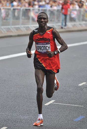
Olympic Marathon Data

Gold medal times for Olympic Marathon since 1896. Marathons before 1924 didn’t have a standardized distance. Present results using pace per km. In 1904 Marathon was badly organized leading to very slow times.

Image from Wikimedia Commons http://bit.ly/16kMKHQ

Olympic Marathon Data

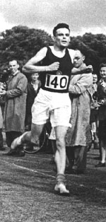
Alan Turing

Probability Winning Olympics?

• He was a formidable Marathon runner.
• In 1946 he ran a time 2 hours 46 minutes.
  • That’s a pace of 3.95 min/km.
• What is the probability he would have won an Olympics if one had been held in 1946?

Gaussian Process Fit

Olympic Marathon Data GP

Learning Covariance Parameters

Can we determine covariance parameters from the data?

\[ \mathcal{N}\left(\mathbf{ y}|\mathbf{0},\mathbf{K}\right)=\frac{1}{(2\pi)^\frac{n}{2}{\det{\mathbf{K}}^{\frac{1}{2}}}}{\exp\left(-\frac{\mathbf{ y}^{\top}\mathbf{K}^{-1}\mathbf{ y}}{2}\right)} \]

\[ \begin{aligned} \mathcal{N}\left(\mathbf{ y}|\mathbf{0},\mathbf{K}\right)=\frac{1}{(2\pi)^\frac{n}{2}\color{yellow}{\det{\mathbf{K}}^{\frac{1}{2}}}}\color{cyan}{\exp\left(-\frac{\mathbf{ y}^{\top}\mathbf{K}^{-1}\mathbf{ y}}{2}\right)} \end{aligned} \]

\[ \begin{aligned} \log \mathcal{N}\left(\mathbf{ y}|\mathbf{0},\mathbf{K}\right)=&\color{yellow}{-\frac{1}{2}\log\det{\mathbf{K}}}\color{cyan}{-\frac{\mathbf{ y}^{\top}\mathbf{K}^{-1}\mathbf{ y}}{2}} \\ &-\frac{n}{2}\log2\pi \end{aligned} \]

\[ E(\boldsymbol{ \theta}) = \color{yellow}{\frac{1}{2}\log\det{\mathbf{K}}} + \color{cyan}{\frac{\mathbf{ y}^{\top}\mathbf{K}^{-1}\mathbf{ y}}{2}} \]

Capacity Control through the Determinant

The parameters are inside the covariance function (matrix). \[k_{i, j} = k(\mathbf{ x}_i, \mathbf{ x}_j; \boldsymbol{ \theta})\]

Eigendecomposition of Covariance

\[\mathbf{K}= \mathbf{R}\boldsymbol{ \Lambda}^2 \mathbf{R}^\top\]

\(\boldsymbol{ \Lambda}\) represents distance on axes. \(\mathbf{R}\) gives rotation.

Eigendecomposition of Covariance

• \(\boldsymbol{ \Lambda}\) is diagonal, \(\mathbf{R}^\top\mathbf{R}= \mathbf{I}\).
• Useful representation since \(\det{\mathbf{K}} = \det{\boldsymbol{ \Lambda}^2} = \det{\boldsymbol{ \Lambda}}^2\).

Capacity control: \(\color{yellow}{\log \det{\mathbf{K}}}\)

❮ ❯

Quadratic Data Fit

Data Fit: \(\color{cyan}{\frac{\mathbf{ y}^\top\mathbf{K}^{-1}\mathbf{ y}}{2}}\)

❮ ❯

\[E(\boldsymbol{ \theta}) = \color{yellow}{\frac{1}{2}\log\det{\mathbf{K}}}+\color{cyan}{\frac{\mathbf{ y}^{\top}\mathbf{K}^{-1}\mathbf{ y}}{2}}\]

Data Fit Term

❮ ❯

Della Gatta Gene Data

• Given given expression levels in the form of a time series from Della Gatta et al. (2008).

Della Gatta Gene Data

Gene Expression Example

• Want to detect if a gene is expressed or not, fit a GP to each gene Kalaitzis and Lawrence (2011).

TP53 Gene Data GP

TP53 Gene Data GP

TP53 Gene Data GP

Multiple Optima

Example: Prediction of Malaria Incidence in Uganda

• Work with Ricardo Andrade Pacheco, John Quinn and Martin Mubangizi (Makerere University, Uganda)
• See AI-DEV Group.
• See UN Global Pulse Disease Outbreaks Site

Malaria Prediction in Uganda

Kapchorwa District

Tororo District

Malaria Prediction in Nagongera (Sentinel Site)

Mubende District

Malaria Prediction in Uganda

GP School at Makerere

Kabarole District

Early Warning System

Early Warning Systems

Additive Covariance

Gelman Book

Basis Function Covariance

Brownian Covariance

MLP Covariance

RELU Covariance

Sinc Covariance

Polynomial Covariance

Periodic Covariance

Linear Model of Coregionalization Covariance

Intrinsic Coregionalization Model Covariance

Extensions

• Approximate inference (e.g. Nickisch and Rasmussen, 2008)
• Large Data (e.g. Bui et al., 2017; Hensman et al., n.d.)
• Multiple outputs (e.g. Álvarez et al., 2012)
• Bayesian optimisation (e.g. Snoek et al., 2012)
• Deep GPs (e.g. Damianou and Lawrence, 2013)