Multifidelity Modelling
An Introduction to Multi-fidelity Modeling in Emukit
Overview
The Data Challenge
- Limited data in environmental sciences & engineering
- Expensive/infeasible physical experiments
- Time-consuming computer simulations
- Examples: Aerospace, nautical engineering, climate modeling
Simulators as a Solution
- Use of simulators to generate data
- More accessible data points
- Example: Computational Fluid Dynamics (CFD)
- Challenge: difficult to simulate accurately contains bias/noise
Multi-fidelity Modeling
- Combining different quality data sources
- High-fidelity: Close to “true” but expensive/limited observations
- Low-fidelity: Abundant but approximate data
- Systematic combination for better predictions
- Support for multiple fidelity levels
Linear multi-fidelity model
\[ f_{\text{high}}(x) = f_{\text{err}}(x) + \rho \,f_{\text{low}}(x) \]
\[ f_{t}(x) = f_{t}(x) + \rho_{t-1} \,f_{t-1}(x), \quad t=1,\dots, T \]
\[ \begin{pmatrix} \mathbf{X}_{\text{low}} \\ \mathbf{X}_{\text{high}} \end{pmatrix} \]
\[ \begin{bmatrix} f_{\text{low}}\left(h\right)\\ f_{\text{high}}\left(h\right) \end{bmatrix} \sim GP \begin{pmatrix} \begin{bmatrix} 0 \\ 0 \end{bmatrix}, \begin{bmatrix} k_{\text{low}} & \rho k_{\text{low}} \\ \rho k_{\text{low}} & \rho^2 k_{\text{low}} + k_{\text{err}} \end{bmatrix} \end{pmatrix} \]
Linear multi-fidelity modeling in Emukit
\[ \mathbf{X}= \begin{pmatrix} x_{\text{low};0}^0 & x_{\text{low};0}^1 & x_{\text{low};0}^2 & 0\\ x_{\text{low};1}^0 & x_{\text{low};1}^1 & x_{\text{low};1}^2 & 0\\ x_{\text{low};2}^0 & x_{\text{low};2}^1 & x_{\text{low};2}^2 & 0\\ x_{\text{high};0}^0 & x_{\text{high};0}^1 & x_{\text{high};0}^2 & 1\\ x_{\text{high};1}^0 & x_{\text{high};1}^1 & x_{\text{high};1}^2 & 1 \end{pmatrix}\quad \mathbf{Y}= \begin{pmatrix} y_{\text{low};0}\\ y_{\text{low};1}\\ y_{\text{low};2}\\ y_{\text{high};0}\\ y_{\text{high};1} \end{pmatrix} \]
Multifidelity Fit
Comparison to standard GP
Nonlinear multi-fidelity model
\[ f_{\text{low}}(x) = \sin(8\pi x) \]
\[ f_{\text{high}}(x) = \left(x- \sqrt{2}\right) \, f_{\text{low}}^2 \]
Failure of linear multi-fidelity model
Nonlinear Multi-fidelity model
\[ f_{\text{high}}(x) = \rho( \, f_{\text{low}}(x)) + \delta(x) \]
Deep Gaussian Processes
Stochastic Process Composition
\[\mathbf{ y}= \mathbf{ f}_4\left(\mathbf{ f}_3\left(\mathbf{ f}_2\left(\mathbf{ f}_1\left(\mathbf{ x}\right)\right)\right)\right)\]
- Compose functions together to form more complex functions
- Compose stochastic processes to form more complex stochastic processes
Composing Gaussian Processes
- Compose two Gaussian processes together
- Resulting process is non-Gaussian
Mathematically
Composite multivariate function
\[ \mathbf{g}(\mathbf{ x})=\mathbf{ f}_5(\mathbf{ f}_4(\mathbf{ f}_3(\mathbf{ f}_2(\mathbf{ f}_1(\mathbf{ x}))))). \]
Equivalent to Markov Chain
- Composite multivariate function \[ p(\mathbf{ y}|\mathbf{ x})= p(\mathbf{ y}|\mathbf{ f}_5)p(\mathbf{ f}_5|\mathbf{ f}_4)p(\mathbf{ f}_4|\mathbf{ f}_3)p(\mathbf{ f}_3|\mathbf{ f}_2)p(\mathbf{ f}_2|\mathbf{ f}_1)p(\mathbf{ f}_1|\mathbf{ x}) \]
Why Composition?
Gaussian processes give priors over functions.
Elegant properties:
- e.g. Derivatives of process are also Gaussian distributed (if they exist).
For particular covariance functions they are ‘universal approximators’, i.e. all functions can have support under the prior.
Gaussian derivatives might ring alarm bells.
E.g. a priori they don’t believe in function ‘jumps’.
Stochastic Process Composition
From a process perspective: process composition.
A (new?) way of constructing more complex processes based on simpler components.
GPy: A Gaussian Process Framework in Python
GPy: A Gaussian Process Framework in Python
- BSD Licensed software base.
- Wide availability of libraries, ‘modern’ scripting language.
- Allows us to set projects to undergraduates in Comp Sci that use GPs.
- Available through GitHub https://github.com/SheffieldML/GPy
- Reproducible Research with Jupyter Notebook.
Features
- Probabilistic-style programming (specify the model, not the algorithm).
- Non-Gaussian likelihoods.
- Multivariate outputs.
- Dimensionality reduction.
- Approximations for large data sets.
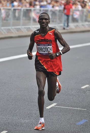
Olympic Marathon Data
|
|
Olympic Marathon Data
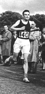
Alan Turing

|
|
Probability Winning Olympics?
- He was a formidable Marathon runner.
- In 1946 he ran a time 2 hours 46 minutes.
- That’s a pace of 3.95 min/km.
- What is the probability he would have won an Olympics if one had been held in 1946?
Gaussian Process Fit
Olympic Marathon Data GP
Deep GP Fit
Can a Deep Gaussian process help?
Deep GP is one GP feeding into another.
Olympic Marathon Data Deep GP
Olympic Marathon Data Deep GP
Olympic Marathon Data Latent 1
Olympic Marathon Data Latent 2
Olympic Marathon Pinball Plot
Deep Emulation
Deep Emulation
Deep Emulation
Deep Emulation
Brief Reflection
- Given you a toolkit of Surrogate Modelling.
- Project work is opportunity to use your imagination.
- Can combine different parts together.
Mountain Car Simulator
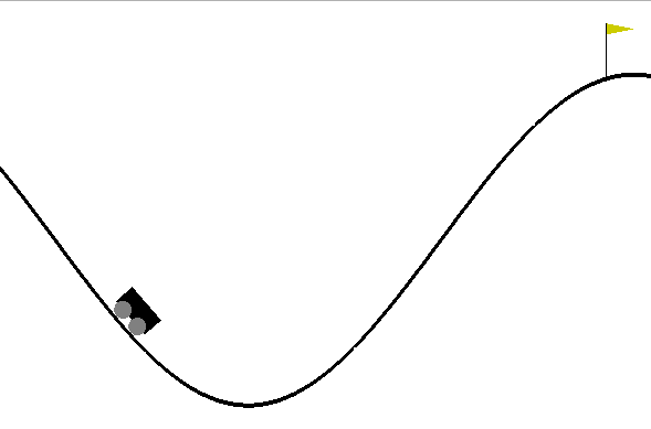
Car Dynamics
\[ \mathbf{ x}_{t+1} = f(\mathbf{ x}_{t},\textbf{u}_{t}) \] where \(\textbf{u}_t\) is the action force, \(\mathbf{ x}_t = (p_t, v_t)\) is the vehicle state
Policy
- Assume policy is linear with parameters \(\boldsymbol{\theta}\) \[ \pi(\mathbf{ x},\theta)= \theta_0 + \theta_p p + \theta_vv. \]
Emulate the Mountain Car
- Goal is find \(\theta\) such that \[ \theta^* = arg \max_{\theta} R_T(\theta). \]
- Reward is computed as 100 for target, minus squared sum of actions
Random Linear Controller
Best Controller after 50 Iterations of Bayesian Optimization
Data Efficient Emulation
- For standard Bayesian Optimization ignored dynamics of the car.
- For more data efficiency, first emulate the dynamics.
- Then do Bayesian optimization of the emulator.
\[ \mathbf{ x}_{t+1} =g(\mathbf{ x}_{t},\textbf{u}_{t}) \]
- Use a Gaussian process to model \[ \Delta v_{t+1} = v_{t+1} - v_{t} \] and \[ \Delta x_{t+1} = p_{t+1} - p_{t} \]
- Two processes, one with mean \(v_{t}\) one with mean \(p_{t}\)
Emulator Training
- Used 500 randomly selected points to train emulators.
- Can make proces smore efficient through experimental design.
Comparison of Emulation and Simulation
Data Efficiency
- Our emulator used only 500 calls to the simulator.
- Optimizing the simulator directly required 37,500 calls to the simulator.
Best Controller using Emulator of Dynamics
Mountain Car: Multi-Fidelity Emulation
\[ f_i\left(\mathbf{ x}\right) = \rho f_{i-1}\left(\mathbf{ x}\right) + \delta_i\left(\mathbf{ x}\right), \]
\[ f_i\left(\mathbf{ x}\right) = g_{i}\left(f_{i-1}\left(\mathbf{ x}\right)\right) + \delta_i\left(\mathbf{ x}\right), \]
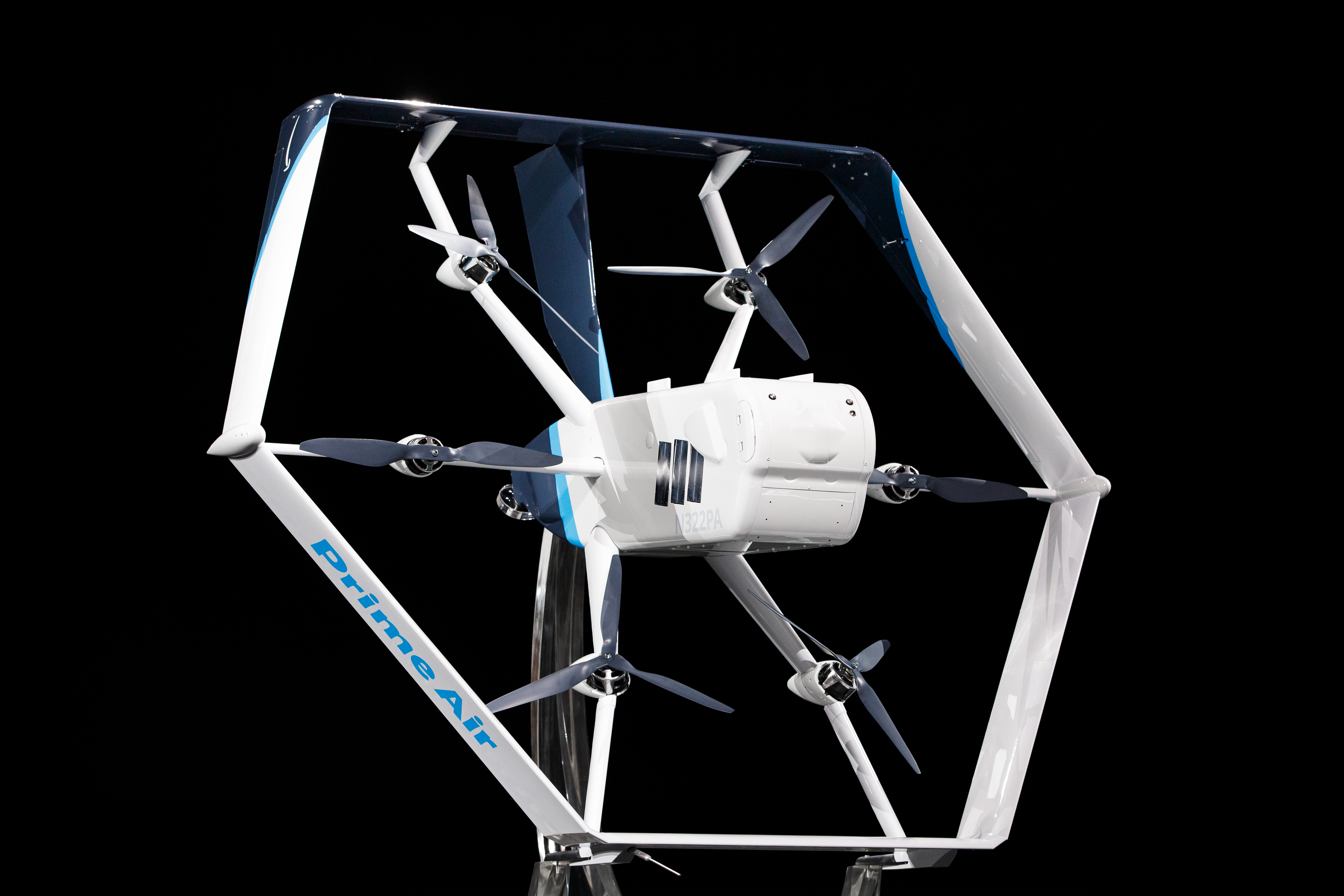
Prime Air
Thanks!
book: The Atomic Human
twitter: @lawrennd
podcast: The Talking Machines
newspaper: Guardian Profile Page
blog posts: