Sensitivity Analysis

Emukit Sensitivity Analysis

A possible definition of sensitivity analysis is the following: The study of how uncertainty in the output of a model (numerical or otherwise) can be apportioned to different sources of uncertainty in the model input (Saltelli et al., 2004). A related practice is ‘uncertainty analysis’, which focuses rather on quantifying uncertainty in model output. Ideally, uncertainty and sensitivity analyses should be run in tandem, with uncertainty analysis preceding in current practice.

In Chapter 1 of Saltelli et al. (2008)

Local Sensitivity

\[ \frac{\partial}{\partial x_i} g(\mathbf{ x}). \]

Global Sensitivity Analysis

\[ \text{var}\left(g(\mathbf{ x})\right) = \left\langle g(\mathbf{ x})^2 \right\rangle _{p(\mathbf{ x})} - \left\langle g(\mathbf{ x}) \right\rangle _{p(\mathbf{ x})}^2, \]

\[ \left\langle h(\mathbf{ x}) \right\rangle _{p(\mathbf{ x})} = \int_\mathbf{ x}h(\mathbf{ x}) p(\mathbf{ x}) \text{d}\mathbf{ x} \]

Input Density

\[ p(\mathbf{ x}) = \prod_{i=1}^pp(x_i) \]

\[ x_i \sim \mathcal{U}\left(0,1\right). \]

Hoeffding-Sobol Decomposition

\[ \begin{align*} g(\mathbf{ x}) = & g_0 + \sum_{i=1}^pg_i(x_i) + \sum_{i<j}^{p} g_{ij}(x_i,x_j) + \cdots \\ & + g_{1,2,\dots,p}(x_1,x_2,\dots,x_p), \end{align*} \]

\[ g_0 = \left\langle g(\mathbf{ x}) \right\rangle _{p(\mathbf{ x})} \]

\[ g_i(x_i) = \left\langle g(\mathbf{ x}) \right\rangle _{p(\mathbf{ x}_{\sim i})} - g_0, \]

\[ p(\mathbf{ x}_{\sim i}) = \int p(\mathbf{ x}) \text{d}x_i \]

\[ g_{i,j}(x_i, x_j) = \left\langle g(\mathbf{ x}) \right\rangle _{p(\mathbf{ x}_{\sim i,j})} - g_i(x_i) - g_j(x_j) - g_0 \]

\[ \begin{align*} \text{var}(g) = & \left\langle g(\mathbf{ x})^2 \right\rangle _{p(\mathbf{ x})} - \left\langle g(\mathbf{ x}) \right\rangle _{p(\mathbf{ x})}^2 \\ = & \left\langle g(\mathbf{ x})^2 \right\rangle _{p(\mathbf{ x})} - g_0^2\\ = & \sum_{i=1}^p\text{var}\left(g_i(x_i)\right) + \sum_{i<j}^{p} \text{var}\left(g_{ij}(x_i,x_j)\right) + \cdots \\ & + \text{var}\left(g_{1,2,\dots,p}(x_1,x_2,\dots,x_p)\right). \end{align*} \]

Sobol Indices

\[ S_\ell = \frac{\text{var}\left(g(\mathbf{ x}_\ell)\right)}{\text{var}\left(g(\mathbf{ x})\right)}, \]

Example: the Ishigami function

Ishigami Function

\[ g(\textbf{x}) = \sin(x_1) + a \sin^2(x_2) + b x_3^4 \sin(x_1). \]

Total Variance

First Order Sobol Indices using Monte Carlo

\[ S_i = \frac{\text{var}\left(g_i(x_i)\right)}{\text{var}\left(g(\mathbf{ x})\right)}. \]

Total Effects Using Monte Carlo

Computing the Sensitivity Indices Using the Output of a Model

Conclusions

• Sobol indices tool for explaining variance of output as coponents of input variables.

Catapult Simulation

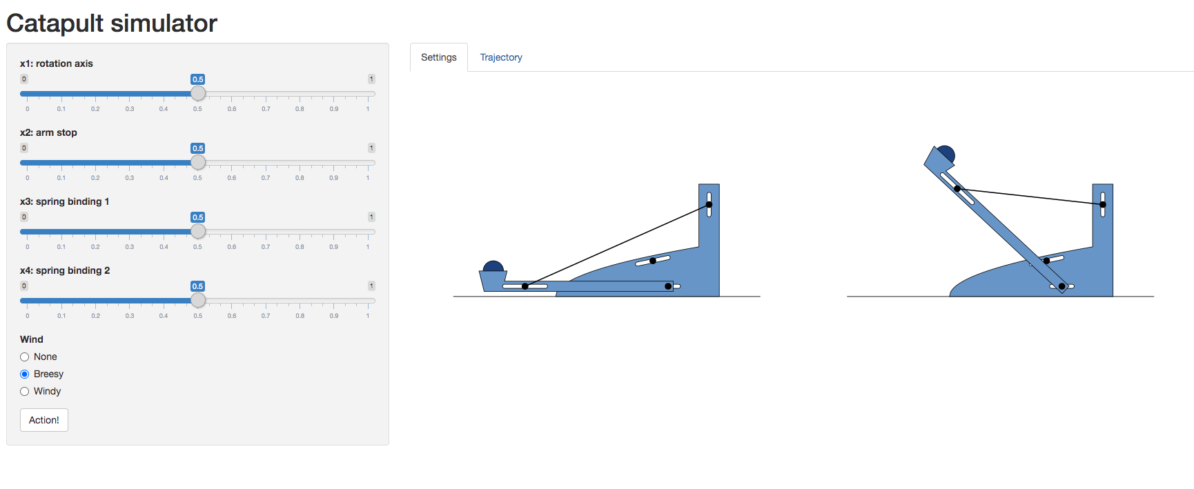
\[ \mathbf{ x}_i = \begin{bmatrix} \texttt{rotation_axis} \\ \texttt{arm_stop} \\ \texttt{spring_binding_1} \\ \texttt{spring_binding_2} \end{bmatrix} \]

Experimental Design for the Catapult

• First build an experimental design loop.
• Start with model free design.
  • Random design
  • Latin hypercube sambling
  • Sobol sequences
  • Orthogonal design

Model Based Design

• Use integrated variance reduction.
• Try afterwards with uncertainty sampling.

Sensitivity Analysis of a Catapult Simulation