Emukit and Experimental Design

Uncertainty Quantification and Design of Experiments

• History of interest, see e.g. McKay et al. (1979)
• The review:
  • Random Sampling
  • Stratified Sampling
  • Latin Hypercube Sampling
• As approaches for Monte Carlo estimates

Random Sampling

{Random sampling is the default approach, this is where across the input domain of interest, we just choose to select samples randomly (perhaps uniformly, or if we believe there’s an underlying distribution

Let the input values \(\mathbf{ x}_1, \dots, \mathbf{ x}_n\) be a random sample from \(f(\mathbf{ x})\). This method of sampling is perhaps the most obvious, and an entire body of statistical literature may be used in making inferences regarding the distribution of \(Y(t)\).

Stratified Sampling

Using stratified sampling, all areas of the sample space of \(\mathbf{ x}\) are represented by input values. Let the sample space \(S\) of \(\mathbf{ x}\) be partitioned into \(I\) disjoint strata \(S_t\). Let \(\pi = P(\mathbf{ x}\in S_i)\) represent the size of \(S_i\). Obtain a random sample \(\mathbf{ x}_{ij}\), \(j = 1, \dots, n\) from \(S_i\). Then of course the \(n_i\) sum to \(n\). If \(I = 1\), we have random sampling over the entire sample space.

Latin Hypercube Sampling

The same reasoning that led to stratified sampling, ensuring that all portions of \(S\) were sampled, could lead further. If we wish to ensure also that each of the input variables \(\mathbf{ x}_k\) has all portions of its distribution represented by input values, we can divide the range of each \(\mathbf{ x}_k\) into \(n\) strata of equal marginal probability \(1/n\), and sample once from each stratum. Let this sample be \(\mathbf{ x}_{kj}\), \(j = 1, \dots, n\). These form the \(\mathbf{ x}_k\) component, \(k = 1, \dots , K\), in \(\mathbf{ x}_i\), \(i = 1, \dots, n\). The components of the various \(\mathbf{ x}_k\)’s are matched at random. This method of selecting input values is an extension of quota sampling (Steinberg 1963), and can be viewed as a \(K\)-dimensional extension of Latin square sampling (Raj 1968).

Emukit

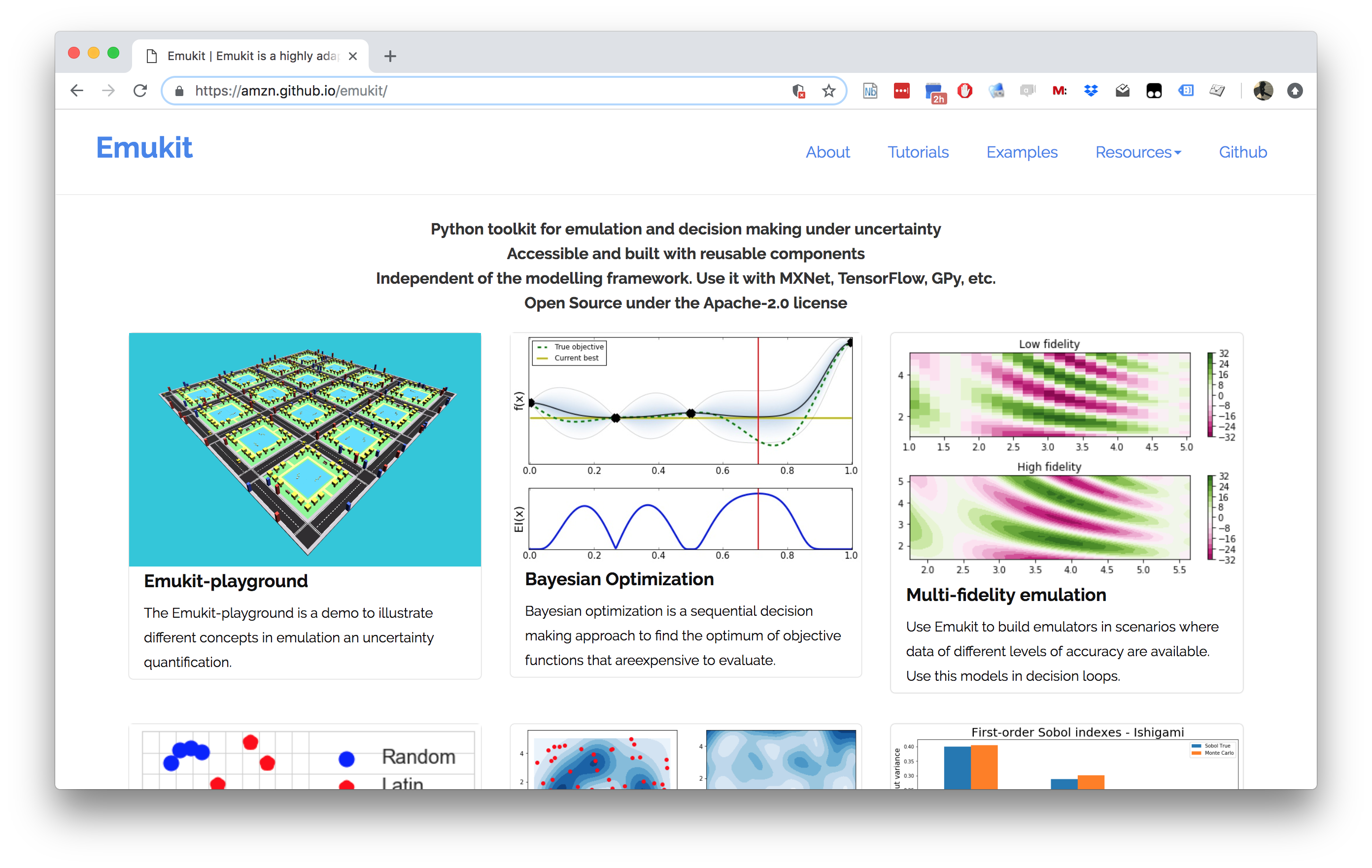
Emukit

Emukit

• Led by: Javier Gonzalez and Andrei Paleyes
  • Team: Mark Pullin, Maren Mahsereci, Alex Gessner, Aaron Klein, Henry Moss and David-Elias Künstle.
  • Management: Cliff McCollum & Neil
• Available on Github
  • Example sensitivity notebook, documentation https://emukit.readthedocs.io/en/latest/

Modular Design

Introduce your own surrogate models.

from emukit.model_wrappers import GPyModelWrapper

To building your own model see this notebook.

from emukit.model_wrappers import YourModelWrapperHere

Structure

• loop
• model
• candidate point calculator
• acquisition
• acquisition optimizer
• user function
• model updater
• stopping condition

Emukit Vision

Emukit and Emulation

Methods

• The different methods: Bayesian optimization, experimental design.

Models

• The probabilistic model that will be used to emulate. Emukit doesn’t define these, the user brings their own.

Tasks

• Still in development: High level goals that owners of the process/simulator might be actually interested in. Examples: measure quality of a simulator, explain complex system behavior.

Structure

while stopping condition is not met:
    optimize acquisition function
    evaluate user function
    update model with new observation

Loop

• An abstract class where the different components come together.

Model

• The surrogate model or emulator, often a Gaussian process.

Candidate Point Calculator

• The routine that combines acquisition with optimizer to compute the next candidate point (or points).

Acquisition

• Our acquisition function: in Bayesian Optimization, this might be Expected Improvement.

Acquisition Optimizer

• The optimization routine we use to optimize the acquisition function. (often this is a non-linear optimizer like L-BFGS (Byrd et al., 1995))

User Function

• The function we’re trying to reason about.

Model Updater

• How to update our surrogate model when we have new training data.

Stopping Condition

• How to decide when to stop our cycle of data acquisition from the target function.

Emukit Tutorial

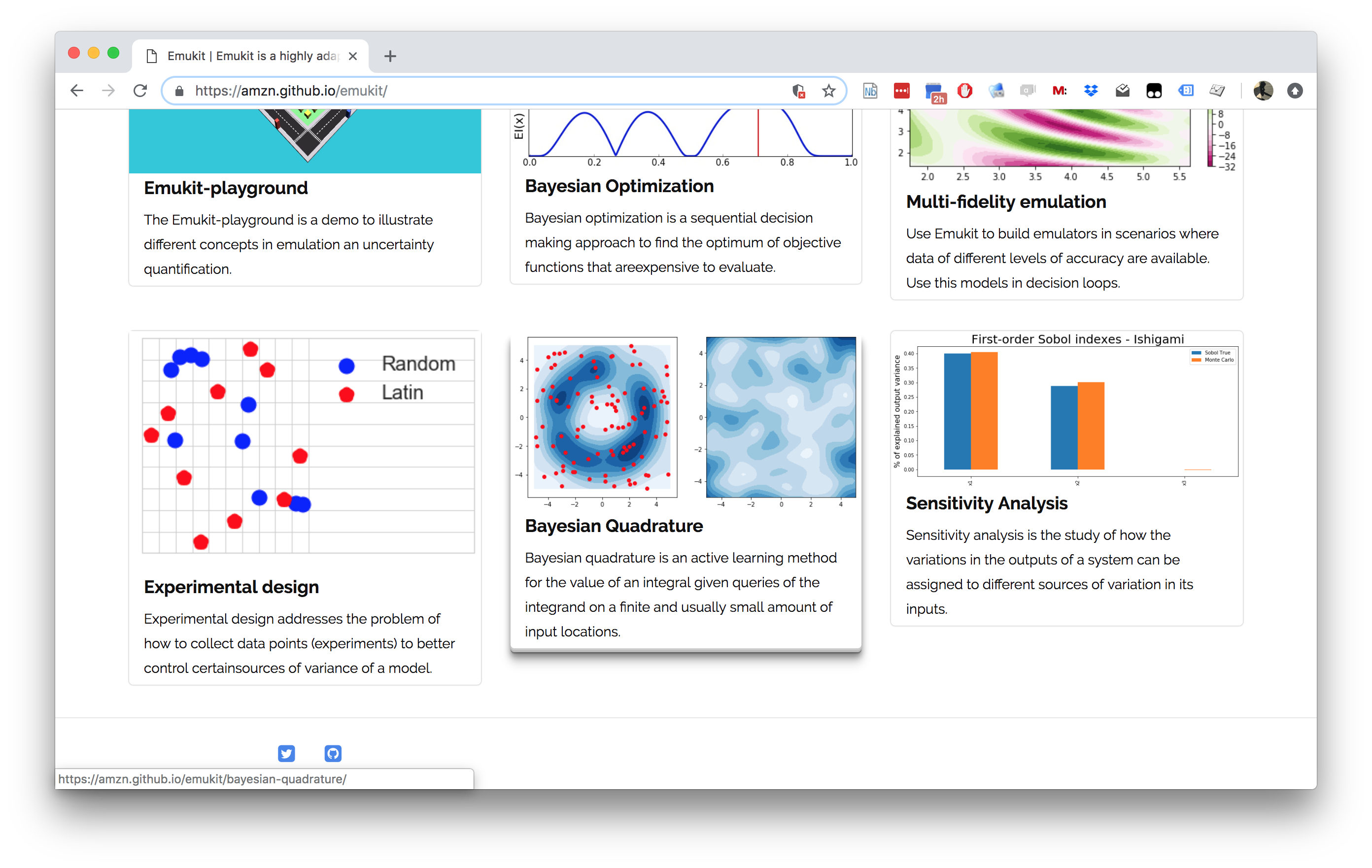
Emukit Overview Summary

• Multi-fidelity emulation: build surrogate models for multiple sources of information;
• Bayesian optimisation: optimise physical experiments and tune parameters ML algorithms;
• Experimental design/Active learning: design experiments and perform active learning with ML models;
• Sensitivity analysis: analyse the influence of inputs on the outputs
• Bayesian quadrature: compute integrals of functions that are expensive to evaluate.

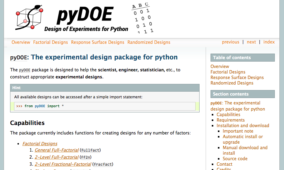
Model Free Experimental Design

Design of Experiments in Python

https://pythonhosted.org/pyDOE/

Experimental Design in Emukit

Forrester Function

Alex Forrester

The Forrester Function

\[ f(x) = (6x-2)^2\sin(12 x-4). \]

Initial Design

The Model

The Acquisition Function

Uncertainty Sampling

\[ a_{US}(\mathbf{ x}) = \sigma^2(\mathbf{ x}). \]

Integrated Variance Reduction

\[ \begin{align*} a_{\text{IVR}} & = \int_{\mathbb{X}}[\sigma^2(\mathbf{ x}') - \sigma^2(\mathbf{ x}'; \mathbf{ x})]\text{d}\mathbf{ x}' \\ & \approx \frac{1}{\# \text{samples}}\sum_i^{\# \text{samples}}[\sigma^2(\mathbf{ x}_i) - \sigma^2(\mathbf{ x}_i; \mathbf{ x})]. \end{align*} \]

\[ a_{LCB} \approx \frac{1}{\# \text{samples}}\sum_i^{\# \text{samples}}\frac{k^2(\mathbf{ x}_i, \mathbf{ x})}{\sigma^2(\mathbf{ x})}. \]

Evaluating the objective function

Add the New Point

y_new = target_function(x_new)
X = np.append(X_init, x_new, axis=0)
Y = np.append(Y_init, y_new, axis=0)
emukit_model.set_data(X, Y)

The Model is Updated

Emukit’s Experimental Design Interface

from emukit.experimental_design.experimental_design_loop import ExperimentalDesignLoop
ed = ExperimentalDesignLoop(space=space, model=emukit_model)
ed.run_loop(target_function, 10)

Conclusions

• Emukit software.
• Example around experimental design.
• Sequential decision making with acquisiton functions.
• Generalizes from the BayesOpt process (e.g. GPyOpt)