Emulation

Emulation

‘I checked it very thoroughly,’ said the computer, ‘and that quite definitely is the answer. I think the problem, to be quite honest with you, is that you’ve never actually known what the question is.’

Douglas Adams The Hitchhiker’s Guide to the Galaxy, 1979, Chapter 28

When you are a Bear of Very Little Brain, and you Think of Things, you find sometimes that a Thing which seemed very Thingish inside you is quite different when it gets out into the open and has other people looking at it.

A.A. Milne as Winnie-the-Pooh in The House at Pooh Corner, 1928

Surrogate Modelling in Practice

• Emergent phenomena require computational power.
• In surrogate modelling we use statistical/ML models to learn regularities in those emergent phenomena.

Types of Simulations

• Simulation can be differential equation models
  • Either abstracted (like epidemilogical models).
  • Or fine-grained (like climate/weather).
• Discrete event simulations
  • Either turn based (e.g. Game of Life or F1 Strategy Simulations)
  • Or Event based (e.g. Gillespie algorithm for chemical models

Fidelity of the Simulation

• Simulations work at different fidelities.
  • e.g. difference between strategy simulation in F1 and aerodynamics simulation

Epidemiology

Modelling Herd Immunity

\[ \frac{\text{d}{S}}{\text{d}t} = - \beta S (I_1 + I_2). \]

\[ \frac{\text{d}{E_1}}{\text{d}t} = \beta S (I_1 + I_2) - \sigma E_1. \]

\[ \frac{\text{d}{E_2}}{\text{d}t} = \sigma E_1 - \sigma E_2. \]

\[ \frac{\text{d}{I_1}}{\text{d}t} = \sigma E_2 - \gamma I_1, \]

\[ \frac{\text{d}{I_2}}{\text{d}t} = \gamma I_1 - \gamma I_2. \]

\[ \frac{\text{d}R}{\text{d}t} = \gamma I_2. \]

Strategies for Simulation

• Split variables into state variables, parameters and results.
• In herd immunity
  • State variables: susceptible, exposed, infectious, recovered.
  • Parameters: reproduction number, expected lengths of infection, lockdown timings.
  • Results: e.g. total number of deaths

Strategies for Simulation

• Use emulator to map from e.g. parameters to total number of deaths.
• Treat parameters and results of simulator as inputs and outputs for emulator.

.

Backtesting Production Code

• Third type of simulation.
• Counterfactual running of system code.

Alexa

Alexa

Alexa

Speech to Text

Cloud Service: Knowledge Base

Text to Speech

Prime Air

Supply Chain Optimization

Supply Chain Optimization

Forecasting

Inventory and Buying

• Automated buying based on:
  • Supplier lead times.
  • Demand Forecast.
  • Cost basis of the product.

Buying System

Monolithic System

Service Oriented Architecture

Intellectual Debt

Examples in Python

• Simpy

• News Vendor Problem in python (for ordering NFL Replica Jerseys.

• Amazon Supply Chain

• Trolley & Pendulum using sympy (symbolic python)

Examples in Python

• Mountain Car in the OpenAI Gym.

• Hodgkin Huxley by Mark Kramer.

• Formula One Race Simulation in Python by Nick Roth.

• Fluid Dynamics Discretisation of PDEs

• Stress in a connecting rod Discretisation of PDEs

• Network simulation Discrete Event simulation.

• Gillespie Algorithm notebook (in Python 2.7).

Simulation System

Monolithic System

Service Oriented Architecture

Experiment, Analyze, Design

A Vision

We don’t know what science we’ll want to do in five years’ time, but we won’t want slower experiments, we won’t want more expensive experiments and we won’t want a narrower selection of experiments.

What do we want?

• Faster, cheaper and more diverse experiments.
• Better ecosystems for experimentation.
• Data oriented architectures.
• Data maturity assessments.
• Data readiness levels.

Packing Problems

Packing Problems

Packing Problems

Modelling with a Function

• What if question of interest is simple?
• For example in packing problem: what is minimum side length?

Erich Friedman Packing Data

Erich Friedman Packing Data: Squares in Squares

Gaussian Process Fit

Erich Friedman Packing Data GP

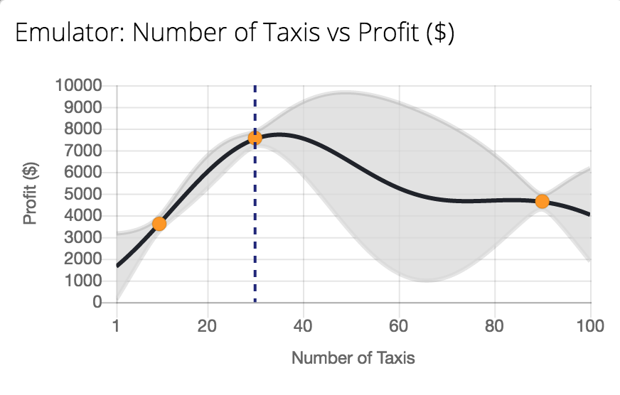
Statistical Emulation

Emulation

Emulation

Emulation

Emulation

Emulation

GPy: A Gaussian Process Framework in Python

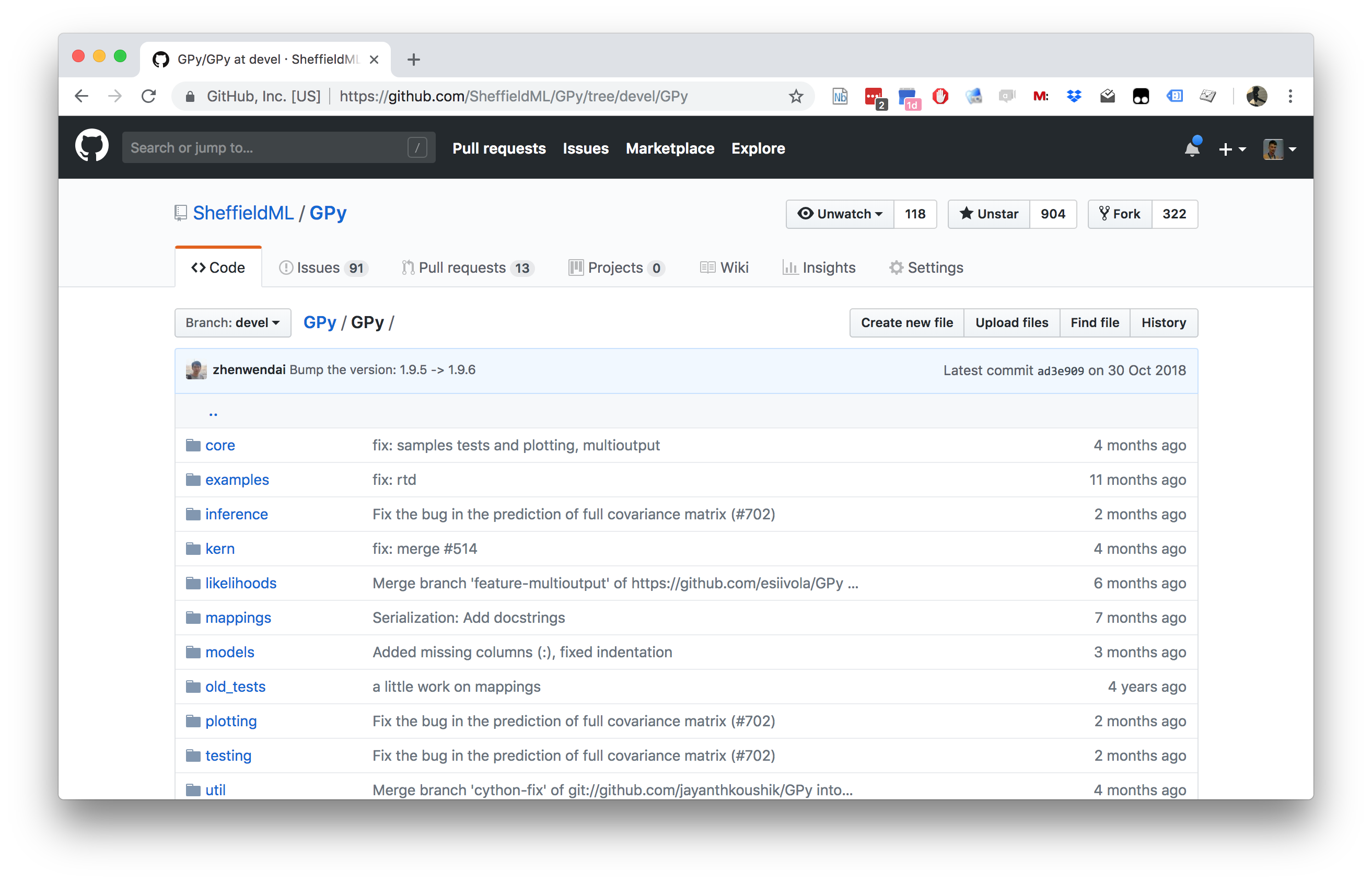
GPy: A Gaussian Process Framework in Python

• BSD Licensed software base.
• Wide availability of libraries, ‘modern’ scripting language.
• Allows us to set projects to undergraduates in Comp Sci that use GPs.
• Available through GitHub https://github.com/SheffieldML/GPy
• Reproducible Research with Jupyter Notebook.

Features

• Probabilistic-style programming (specify the model, not the algorithm).
• Non-Gaussian likelihoods.
• Multivariate outputs.
• Dimensionality reduction.
• Approximations for large data sets.

GPy Tutorial

Covariance Functions

\[ k(\mathbf{ x}, \mathbf{ x}^\prime) = \alpha \exp\left(-\frac{\left\Vert \mathbf{ x}- \mathbf{ x}^\prime \right\Vert_2^2}{2\ell^2}\right), \]

input_dim=1
alpha = 1.0
lengthscale = 2.0
kern = GPy.kern.RBF(input_dim=input_dim, 
                    variance=alpha, 
                    lengthscale=lengthscale)

Kernel Output

Covariance Functions in GPy

• Includes a range of covariance functions
  • E.g. Matern family, Brownian motion, periodic, linear etc.
  • Can define new covariances

Combining Covariance Functions in GPy

kern1 = GPy.kern.RBF(1, variance=1., lengthscale=2.)
kern2 = GPy.kern.Matern52(1, variance=2., lengthscale=4.)
kern = kern1 + kern2

Multiplication

kern1 = GPy.kern.RBF(1, variance=1., lengthscale=2.)
kern2 = GPy.kern.Matern52(1, variance=2., lengthscale=4.)
kern = kern1 * kern2
display(kern)

A Gaussian Process Regression Model

\[ f( x) = − \cos(\pi x) + \sin(4\pi x) \]

\[ y(x) = f(x) + \epsilon, \]

Noisy Sine

kern = GPy.kern.RBF(input_dim=1, variance=1., lengthscale=1.)
model = GPy.models.GPRegression(X,Y,kern)

GP Fit to Noisy Sine

Covariance Function Parameter Estimation

model.optimize(messages=True)

GPy and Emulation

\[ f(\mathbf{ x}) = a(x_2 - bx_1^2 + cx_1 - r)^2 + s(1-t \cos(x_1)) + s \]

Computation of \(\left\langle f(U)\right\rangle\)

• Compute the expectation of the Branin function.
• Sample at 25 points on a grid.
• Compute the mean (Reiemann sum approximation).

Emulate and do MC Samples

Alternatively, we can fit a GP model and compute the integral of the best predictor by Monte Carlo sampling.

Branin Function Fit

Uncertainty Quantification and Design of Experiments

• History of interest, see e.g. McKay et al. (1979)
• The review:
  • Random Sampling
  • Stratified Sampling
  • Latin Hypercube Sampling
• As approaches for Monte Carlo estimates

Random Sampling

{Random sampling is the default approach, this is where across the input domain of interest, we just choose to select samples randomly (perhaps uniformly, or if we believe there’s an underlying distribution

Let the input values \(\mathbf{ x}_1, \dots, \mathbf{ x}_n\) be a random sample from \(f(\mathbf{ x})\). This method of sampling is perhaps the most obvious, and an entire body of statistical literature may be used in making inferences regarding the distribution of \(Y(t)\).

Stratified Sampling

Using stratified sampling, all areas of the sample space of \(\mathbf{ x}\) are represented by input values. Let the sample space \(S\) of \(\mathbf{ x}\) be partitioned into \(I\) disjoint strata \(S_t\). Let \(\pi = P(\mathbf{ x}\in S_i)\) represent the size of \(S_i\). Obtain a random sample \(\mathbf{ x}_{ij}\), \(j = 1, \dots, n\) from \(S_i\). Then of course the \(n_i\) sum to \(n\). If \(I = 1\), we have random sampling over the entire sample space.

Latin Hypercube Sampling

The same reasoning that led to stratified sampling, ensuring that all portions of \(S\) were sampled, could lead further. If we wish to ensure also that each of the input variables \(\mathbf{ x}_k\) has all portions of its distribution represented by input values, we can divide the range of each \(\mathbf{ x}_k\) into \(n\) strata of equal marginal probability \(1/n\), and sample once from each stratum. Let this sample be \(\mathbf{ x}_{kj}\), \(j = 1, \dots, n\). These form the \(\mathbf{ x}_k\) component, \(k = 1, \dots , K\), in \(\mathbf{ x}_i\), \(i = 1, \dots, n\). The components of the various \(\mathbf{ x}_k\)’s are matched at random. This method of selecting input values is an extension of quota sampling (Steinberg 1963), and can be viewed as a \(K\)-dimensional extension of Latin square sampling (Raj 1968).

Emukit Playground

• Work Leah Hirst, Software Engineering Intern and Cliff McCollum.

• Tutorial on emulation.

Emukit Playground

Emukit Playground

Conclusions

• Characterised types of simulation.
  • Physical laws
  • Discrete event
  • Production Software Systems
• Introduced notion of emulation to replace simulation.
• Overviewed GPy software.