Week 5: Multifidelity Modelling

[jupyter][google colab][reveal]

Neil D. Lawrence

Abstract:

This week we introduce multifidelity modelling. We use surrogate models to capture different qualities of information from different simulations.

Setup

notutils

This small package is a helper package for various notebook utilities used below.

The software can be installed using

%pip install notutils

from the command prompt where you can access your python installation.

The code is also available on GitHub: https://github.com/lawrennd/notutils

Once notutils is installed, it can be imported in the usual manner.

import notutils

pods

In Sheffield we created a suite of software tools for ‘Open Data Science’. Open data science is an approach to sharing code, models and data that should make it easier for companies, health professionals and scientists to gain access to data science techniques.

You can also check this blog post on Open Data Science.

The software can be installed using

%pip install pods

from the command prompt where you can access your python installation.

The code is also available on GitHub: https://github.com/lawrennd/ods

Once pods is installed, it can be imported in the usual manner.

import pods

mlai

The mlai software is a suite of helper functions for teaching and demonstrating machine learning algorithms. It was first used in the Machine Learning and Adaptive Intelligence course in Sheffield in 2013.

The software can be installed using

%pip install mlai

from the command prompt where you can access your python installation.

The code is also available on GitHub: https://github.com/lawrennd/mlai

Once mlai is installed, it can be imported in the usual manner.

import mlai

%pip install gpy

%pip install pyDOE

%pip install emukit

An Introduction to Multi-fidelity Modeling in Emukit

A reminder from our lecture on Emulation. This diagram implies that we might expect our statistical emulator to be able to ‘adjudicate’ between simulations with different fidelity.

Figure: A statistical emulator is a system that reconstructs the simulation with a statistical model. As well as reconstructing the simulation, a statistical emulator can be used to correlate with the real world.

Overview

This section is based on the Emukit multifidelity tutorial found here and written by Javier Gonzalez, Mark Pullin, Oleg Ponomarev and David-Elias Künstle.

A common issue encountered when applying machine learning to environmental sciences and engineering problems is the difficulty or cost required to obtain sufficient data for building robust models. Possible examples include aerospace and nautical engineering, where it is both infeasible and prohibitively expensive to run a vast number of experiments using the actual vehicle. Even when there is no physical artifact involved, such as in climate modeling, data may still be hard to obtain when these can only be collected by running an expensive computer experiment, where the time required to acquire an individual data sample restricts the volume of data that can later be used for modeling.

Constructing a reliable model when only few observations are available is challenging, which is why it is common practice to develop simulators of the actual system, from which data points can be more easily obtained. In engineering applications, such simulators often take the form of Computational Fluid Dynamics (CFD) tools which approximate the behaviour of the true artifact for a given design or configuration. However, although it is now possible to obtain more data samples, it is highly unlikely that these simulators model the true system exactly; instead, these are expected to contain some degree of bias and/or noise.

From the above, one can deduce that naively combining observations from multiple information sources could result in the model giving biased predictions which do not accurately reflect the true problem. To this end, multi-fidelity models are designed to augment the limited true observations available with cheaply-obtained approximations in a principled manner. In such models, observations obtained from the true source are referred to as high-fidelity observations, whereas approximations are denoted as being low-fidelity. These low-fidelity observations are then systemically combined with the more accurate (but limited) observations in order to predict the high-fidelity output more effectively. Note than we can generally combine information from multiple lower fidelity sources, which can all be seen as auxiliary tasks in support of a single primary task.

In this notebook, we shall investigate a selection of multi-fidelity models based on Gaussian processes which are readily available in EmuKit. We start by investigating the traditional linear multi-fidelity model as proposed in (Kennedy and O’Hagan, 2000). Subsequently, we shall illustrate why this model can be unsuitable when the mapping from low to high-fidelity observations is nonlinear, and demonstrate how an alternate model proposed in Paris Perdikaris et al. (2017) can alleviate this issue. The examples presented in this notebook can then be easily adapted to a variety of problem settings.

Linear multi-fidelity model

The linear multi-fidelity model proposed in Kennedy and O’Hagan (2000) is widely viewed as a reference point for all such models. In this model, the high-fidelity (true) function is modeled as a scaled sum of the low-fidelity function plus an error term: \[ f_{\text{high}}(x) = f_{\text{err}}(x) + \rho \,f_{\text{low}}(x) \] In this equation, \(f_{\text{low}}(x)\) is taken to be a Gaussian process modeling the outputs of the lower fidelity function, while \(\rho\) is a scaling factor indicating the magnitude of the correlation to the high-fidelity data. Setting this to 0 implies that there is no correlation between observations at different fidelities. Meanwhile, \(f_{\text{err}}(x)\) denotes yet another Gaussian process which models the bias term for the high-fidelity data. Note that \(f_{\text{err}}(x)\) and \(f_{\text{low}}(x)\) are assumed to be independent processes which are only related by the equation given above.

Note: While we shall limit our explanation to the case of two fidelities, this set-up can easily be generalized to cater for \(T\) fidelities as follows: \[ f_{t}(x) = f_{t}(x) + \rho_{t-1} \,f_{t-1}(x), \quad t=1,\dots, T \]

If the training points are sorted such that the low and high-fidelity points are grouped together: \[ \begin{pmatrix} \mathbf{X}_{\text{low}} \\ \mathbf{X}_{\text{high}} \end{pmatrix} \]

we can express the model as a single Gaussian process having the following prior. \[ \begin{bmatrix} f_{\text{low}}\left(h\right)\\ f_{\text{high}}\left(h\right) \end{bmatrix} \sim GP \begin{pmatrix} \begin{bmatrix} 0 \\ 0 \end{bmatrix}, \begin{bmatrix} k_{\text{low}} & \rho k_{\text{low}} \\ \rho k_{\text{low}} & \rho^2 k_{\text{low}} + k_{\text{err}} \end{bmatrix} \end{pmatrix} \]

Linear multi-fidelity modeling in Emukit

As a first example of how the linear multi-fidelity model implemented in Emukit emukit.multi_fidelity.models.GPyLinearMultiFidelityModel can be used, we shall consider the two-fidelity Forrester function. This benchmark is frequently used to illustrate the capabilities of multi-fidelity models.

import numpy as np

np.random.seed(20)

import GPy
import emukit.multi_fidelity
import emukit.test_functions
from emukit.model_wrappers.gpy_model_wrappers import GPyMultiOutputWrapper
from emukit.multi_fidelity.models import GPyLinearMultiFidelityModel

Generate samples from the Forrester function

high_fidelity = emukit.test_functions.forrester.forrester
low_fidelity = emukit.test_functions.forrester.forrester_low

x_plot = np.linspace(0, 1, 200)[:, np.newaxis]
y_plot_l = low_fidelity(x_plot)
y_plot_h = high_fidelity(x_plot)

x_train_l = np.atleast_2d(np.random.rand(12)).T
x_train_h = np.atleast_2d(np.random.permutation(x_train_l)[:6])
y_train_l = low_fidelity(x_train_l)
y_train_h = high_fidelity(x_train_h)

The inputs to the models are expected to take the form of ndarrays where the last column indicates the fidelity of the observed points.

Although only the input points, \(X\), are augmented with the fidelity level, the observed outputs \(Y\) must also be converted to array form.

For example, a dataset consisting of 3 low-fidelity points and 2 high-fidelity points would be represented as follows, where the input is three-dimensional while the output is one-dimensional: \[ \mathbf{X}= \begin{pmatrix} x_{\text{low};0}^0 & x_{\text{low};0}^1 & x_{\text{low};0}^2 & 0\\ x_{\text{low};1}^0 & x_{\text{low};1}^1 & x_{\text{low};1}^2 & 0\\ x_{\text{low};2}^0 & x_{\text{low};2}^1 & x_{\text{low};2}^2 & 0\\ x_{\text{high};0}^0 & x_{\text{high};0}^1 & x_{\text{high};0}^2 & 1\\ x_{\text{high};1}^0 & x_{\text{high};1}^1 & x_{\text{high};1}^2 & 1 \end{pmatrix}\quad \mathbf{Y}= \begin{pmatrix} y_{\text{low};0}\\ y_{\text{low};1}\\ y_{\text{low};2}\\ y_{\text{high};0}\\ y_{\text{high};1} \end{pmatrix} \] This is a representation we first developed for the GPy software. It allows for a lot of flexibility for Gaussian processes that describe multiple correlated functions, like the ‘multi-fidelity’ model of Kennedy and O’Hagan (2000).

As an aside there is quite a lot of history to modelling Gaussian processes which represent multiple output functions. Back in 2009, with Mauricio Alvarez, we organized a series of workshops where we worked across the geostatistics, the emulation and the machine learning communities to build understanding. You can see details of the first of these workshops (held in Manchester) here. The second of these workshops also integrated ideas from the classical kernel community, and was held at NeurIPS in 2009 in collaboration with Lorenzo Rosasco, you can find the workshop page here. We summarized the conclusions from those meetings in a review paper led by Mauricio, that you can find here (Álvarez et al., 2012).

In that terminology the multifidelity model we’re using here is known as a “intrinsic coregionalisation model” and it is one of the simplest types of multi-output Gaussian processes you can build.

Mauricio’s thesis (Álvarez, 2011) focused on particular multiple output covariances derived from physical information embedded in the system, such as differential equations. See e.g., Álvarez et al. (2013) or Lawrence et al. (n.d.) for an application.

A similar procedure must be carried out for obtaining predictions at new test points, whereby the fidelity indicated in the column then indicates the fidelity at which the function must be predicted for a designated point.

For convenience of use, we provide helper methods for easily converting between a list of arrays (ordered from the lowest to the highest fidelity) and the required ndarray representation. This is found in emukit.multi_fidelity.convert_lists_to_array.

Convert lists of arrays to ndarrays augmented with fidelity indicators.

from emukit.multi_fidelity.convert_lists_to_array import convert_x_list_to_array, convert_xy_lists_to_arrays

X_train, Y_train = convert_xy_lists_to_arrays([x_train_l, x_train_h], 
                                                    [y_train_l, y_train_h])

Plot the original functions.

Figure: High and low fidelity Forrester functions.

Observe that in the example above we restrict our observations to 12 from the lower-fidelity function and only 6 from the high-fidelity function. As we shall demonstrate further below, fitting a standard GP model to the few high-fidelity observations is unlikely to result in an acceptable fit, which is why we shall instead consider the linear multi-fidelity model presented in this section.

Below we fit a linear multi-fidelity model to the available low and high-fidelity observations. Given the smoothness of the functions, we opt to use an exponentiated quadratic kernel for both the bias and correlation components of the model.

Note: The model implementation defaults to a MixedNoise noise likelihood whereby there is independent Gaussian noise for each fidelity.

This can be modified upfront using the ‘likelihood’ parameter in the model constructor, or by updating them directly after the model has been created. In the example below, we choose to fix the noise to ‘0’ for both fidelities to reflect that the observations are exact.

Construct a linear multi-fidelity model.

kernels = [GPy.kern.RBF(1), GPy.kern.RBF(1)]
lin_mf_kernel = emukit.multi_fidelity.kernels.LinearMultiFidelityKernel(kernels)
gpy_lin_mf_model = GPyLinearMultiFidelityModel(X_train, Y_train, lin_mf_kernel, n_fidelities=2)
gpy_lin_mf_model.mixed_noise.Gaussian_noise.fix(0)
gpy_lin_mf_model.mixed_noise.Gaussian_noise_1.fix(0)

Wrap the model using the given GPyMultiOutputWrapper

lin_mf_model = GPyMultiOutputWrapper(gpy_lin_mf_model, 2, n_optimization_restarts=5)

Fit the model

lin_mf_model.optimize()

Convert x_plot to its ndarray representation.

X_plot = convert_x_list_to_array([x_plot, x_plot])
X_plot_l = X_plot[:len(x_plot)]
X_plot_h = X_plot[len(x_plot):]

Compute mean predictions and associated variance.

lf_mean_lin_mf_model, lf_var_lin_mf_model = lin_mf_model.predict(X_plot_l)
lf_std_lin_mf_model = np.sqrt(lf_var_lin_mf_model)
hf_mean_lin_mf_model, hf_var_lin_mf_model = lin_mf_model.predict(X_plot_h)
hf_std_lin_mf_model = np.sqrt(hf_var_lin_mf_model)

Plot the posterior mean and variance.

Figure: Linear multi-fidelity model fit to low and high-fidelity Forrester function

The above plot demonstrates how the multi-fidelity model learns the relationship between the low and high-fidelity observations to model both of the corresponding functions.

In this example, the posterior mean almost fits the true function exactly, while the associated uncertainty returned by the model is also appropriately small given the good fit.

Comparison to standard GP

In the absence of such a multi-fidelity model, a regular Gaussian process would have been fit exclusively to the high fidelity data.

As illustrated in the figure below, the resulting Gaussian process posterior yields a much worse fit to the data than that obtained by the multi-fidelity model. The uncertainty estimates are also poorly calibrated.

Create standard GP model using only high-fidelity data.

kernel = GPy.kern.RBF(1)
high_gp_model = GPy.models.GPRegression(x_train_h, y_train_h, kernel)
high_gp_model.Gaussian_noise.fix(0)

Fit the GP model.

high_gp_model.optimize_restarts(5)

Compute mean predictions and associated variance.

hf_mean_high_gp_model, hf_var_high_gp_model  = high_gp_model.predict(x_plot)
hf_std_hf_gp_model = np.sqrt(hf_var_high_gp_model)

Plot the posterior mean and variance for the high-fidelity GP model.

Figure: Comparison of linear multi-fidelity model and high fidelity GP

Nonlinear multi-fidelity model

Although the model described above works well when the mapping between the low and high-fidelity functions is linear, several issues may be encountered when this is not the case.

Consider the following example, where the low and high-fidelity functions are defined as follows: \[ f_{\text{low}}(x) = \sin(8\pi x) \]

\[ f_{\text{high}}(x) = \left(x- \sqrt{2}\right) \, f_{\text{low}}^2 \]

Generate data for nonlinear example.

high_fidelity = emukit.test_functions.non_linear_sin.nonlinear_sin_high
low_fidelity = emukit.test_functions.non_linear_sin.nonlinear_sin_low

x_plot = np.linspace(0, 1, 200)[:, np.newaxis]
y_plot_l = low_fidelity(x_plot)
y_plot_h = high_fidelity(x_plot)

n_low_fidelity_points = 50
n_high_fidelity_points = 14

x_train_l = np.linspace(0, 1, n_low_fidelity_points)[:, np.newaxis]
y_train_l = low_fidelity(x_train_l)

x_train_h = x_train_l[::4, :]
y_train_h = high_fidelity(x_train_h)

Convert lists of arrays to ND-arrays augmented with fidelity indicators

X_train, Y_train = convert_xy_lists_to_arrays([x_train_l, x_train_h], [y_train_l, y_train_h])

Figure: High and low-fidelity functions

In this case, the mapping between the two functions is nonlinear, as can be observed by plotting the high-fidelity observations as a function of the lower fidelity observations.

Figure: Mapping from low-fidelity to high-fidelity.

Failure of linear multi-fidelity model

Below we fit the linear multi-fidelity model to this new problem and plot the results.

Construct a linear multi-fidelity model.

kernels = [GPy.kern.RBF(1), GPy.kern.RBF(1)]
lin_mf_kernel = emukit.multi_fidelity.kernels.LinearMultiFidelityKernel(kernels)
gpy_lin_mf_model = GPyLinearMultiFidelityModel(X_train, Y_train, lin_mf_kernel, n_fidelities=2)
gpy_lin_mf_model.mixed_noise.Gaussian_noise.fix(0)
gpy_lin_mf_model.mixed_noise.Gaussian_noise_1.fix(0)

lin_mf_model = model = GPyMultiOutputWrapper(gpy_lin_mf_model, 2, n_optimization_restarts=5)

Fit the model

lin_mf_model.optimize()

Convert test points to appropriate representation

X_plot = convert_x_list_to_array([x_plot, x_plot])
X_plot_low = X_plot[:200]
X_plot_high = X_plot[200:]

Compute mean and variance predictions

hf_mean_lin_mf_model, hf_var_lin_mf_model = lin_mf_model.predict(X_plot_high)
hf_std_lin_mf_model = np.sqrt(hf_var_lin_mf_model)

Compare linear and nonlinear model fits

Figure: Linear multi-fidelity model fit to high-fidelity function

As expected, the linear multi-fidelity model was unable to capture the nonlinear relationship between the low and high-fidelity data. Consequently, the resulting fit of the true function is also poor.

Nonlinear Multi-fidelity model

In view of the deficiencies of the linear multi-fidelity model, a nonlinear multi-fidelity model is proposed in Paris Perdikaris et al. (2017) to better capture these correlations. This nonlinear model is constructed as follows: \[ f_{\text{high}}(x) = \rho( \, f_{\text{low}}(x)) + \delta(x) \] Replacing the linear scaling factor with a non-deterministic function results in a model which can thus capture the nonlinear relationship between the fidelities.

This model is implemented in Emukit as emukit.multi_fidelity.models.NonLinearModel.

It is defined in a sequential manner where a Gaussian process model is trained for every set of fidelity data available. Once again, we manually fix the noise parameter for each model to 0. The parameters of the two Gaussian processes are then optimized sequentially, starting from the low-fidelity.

Create nonlinear model.

from emukit.multi_fidelity.models.non_linear_multi_fidelity_model import make_non_linear_kernels, NonLinearMultiFidelityModel

base_kernel = GPy.kern.RBF
kernels = make_non_linear_kernels(base_kernel, 2, X_train.shape[1] - 1)
nonlin_mf_model = NonLinearMultiFidelityModel(X_train, Y_train, n_fidelities=2, kernels=kernels, 
                                              verbose=True, optimization_restarts=5)
for m in nonlin_mf_model.models:
    m.Gaussian_noise.variance.fix(0)

nonlin_mf_model.optimize()

Now we compute the mean and variance predictions

hf_mean_nonlin_mf_model, hf_var_nonlin_mf_model = nonlin_mf_model.predict(X_plot_high)
hf_std_nonlin_mf_model = np.sqrt(hf_var_nonlin_mf_model)

lf_mean_nonlin_mf_model, lf_var_nonlin_mf_model = nonlin_mf_model.predict(X_plot_low)
lf_std_nonlin_mf_model = np.sqrt(lf_var_nonlin_mf_model)

Figure: Nonlinear multi-fidelity model fit to low and high-fidelity functions.

Fitting the nonlinear fidelity model to the available data very closely fits the high-fidelity function while also fitting the low-fidelity function exactly. This is a vast improvement over the results obtained using the linear model. We can also confirm that the model is properly capturing the correlation between the low and high-fidelity observations by plotting the mapping learned by the model to the true mapping shown earlier.

Figure: Mapping from low fidelity to high fidelity

Deep Gaussian Processes

These non-linear multi-fidelity models are an example of composing Gaussian processes together. This type of non-linear relationship leads to what we refer to as a Deep Gaussian process (Damianou and Lawrence, 2013; Lawrence and Moore, 2007) which Andreas Damianou worked on for his PhD thesis (Damianou, 2015).

These ideas lead to the notion of ‘deep emulation’, where a number of emulators are chained together to represent a system.

Stochastic Process Composition

\[\mathbf{ y}= \mathbf{ f}_4\left(\mathbf{ f}_3\left(\mathbf{ f}_2\left(\mathbf{ f}_1\left(\mathbf{ x}\right)\right)\right)\right)\]

Mathematically, a deep Gaussian process can be seen as a composite multivariate function, \[ \mathbf{g}(\mathbf{ x})=\mathbf{ f}_5(\mathbf{ f}_4(\mathbf{ f}_3(\mathbf{ f}_2(\mathbf{ f}_1(\mathbf{ x}))))). \] Or if we view it from the probabilistic perspective we can see that a deep Gaussian process is specifying a factorization of the joint density, the standard deep model takes the form of a Markov chain.

\[ p(\mathbf{ y}|\mathbf{ x})= p(\mathbf{ y}|\mathbf{ f}_5)p(\mathbf{ f}_5|\mathbf{ f}_4)p(\mathbf{ f}_4|\mathbf{ f}_3)p(\mathbf{ f}_3|\mathbf{ f}_2)p(\mathbf{ f}_2|\mathbf{ f}_1)p(\mathbf{ f}_1|\mathbf{ x}) \]

Figure: Probabilistically the deep Gaussian process can be represented as a Markov chain. Indeed they can even be analyzed in this way (Dunlop et al., n.d.).

Figure: More usually deep probabilistic models are written vertically rather than horizontally as in the Markov chain.

Why Composition?

If the result of composing many functions together is simply another function, then why do we bother? The key point is that we can change the class of functions we are modeling by composing in this manner. A Gaussian process is specifying a prior over functions, and one with a number of elegant properties. For example, the derivative process (if it exists) of a Gaussian process is also Gaussian distributed. That makes it easy to assimilate, for example, derivative observations. But that also might raise some alarm bells. That implies that the marginal derivative distribution is also Gaussian distributed. If that’s the case, then it means that functions which occasionally exhibit very large derivatives are hard to model with a Gaussian process. For example, a function with jumps in.

A one off discontinuity is easy to model with a Gaussian process, or even multiple discontinuities. They can be introduced in the mean function, or independence can be forced between two covariance functions that apply in different areas of the input space. But in these cases we will need to specify the number of discontinuities and where they occur. In otherwords we need to parameterise the discontinuities. If we do not know the number of discontinuities and don’t wish to specify where they occur, i.e. if we want a non-parametric representation of discontinuities, then the standard Gaussian process doesn’t help.

Stochastic Process Composition

The deep Gaussian process leads to non-Gaussian models, and non-Gaussian characteristics in the covariance function. In effect, what we are proposing is that we change the properties of the functions we are considering by composing stochastic processes. This is an approach to creating new stochastic processes from well known processes.

Additionally, we are not constrained to the formalism of the chain. For example, we can easily add single nodes emerging from some point in the depth of the chain. This allows us to combine the benefits of the graphical modelling formalism, but with a powerful framework for relating one set of variables to another, that of Gaussian processes

Figure: More generally we aren’t constrained by the Markov chain. We can design structures that respect our belief about the underlying conditional dependencies. Here we are adding a side note from the chain.

GPy: A Gaussian Process Framework in Python

Gaussian processes are a flexible tool for non-parametric analysis with uncertainty. The GPy software was started in Sheffield to provide a easy to use interface to GPs. One which allowed the user to focus on the modelling rather than the mathematics.

Figure: GPy is a BSD licensed software code base for implementing Gaussian process models in Python. It is designed for teaching and modelling. We welcome contributions which can be made through the GitHub repository https://github.com/SheffieldML/GPy

GPy is a BSD licensed software code base for implementing Gaussian process models in python. This allows GPs to be combined with a wide variety of software libraries.

The software itself is available on GitHub and the team welcomes contributions.

The aim for GPy is to be a probabilistic-style programming language, i.e., you specify the model rather than the algorithm. As well as a large range of covariance functions the software allows for non-Gaussian likelihoods, multivariate outputs, dimensionality reduction and approximations for larger data sets.

The documentation for GPy can be found here.

This notebook depends on PyDeepGP. This library can be installed via pip.

%pip install --upgrade git+https://github.com/SheffieldML/PyDeepGP.git

# Late bind setup methods to DeepGP object
from mlai.deepgp_tutorial import initialize
from mlai.deepgp_tutorial import staged_optimize
from mlai.deepgp_tutorial import posterior_sample
from mlai.deepgp_tutorial import visualize
from mlai.deepgp_tutorial import visualize_pinball

import deepgp
deepgp.DeepGP.initialize=initialize
deepgp.DeepGP.staged_optimize=staged_optimize
deepgp.DeepGP.posterior_sample=posterior_sample
deepgp.DeepGP.visualize=visualize
deepgp.DeepGP.visualize_pinball=visualize_pinball

Olympic Marathon Data

Gold medal times for Olympic Marathon since 1896. Marathons before 1924 didn’t have a standardized distance. Present results using pace per km. In 1904 Marathon was badly organized leading to very slow times.

Image from Wikimedia Commons http://bit.ly/16kMKHQ

The first thing we will do is load a standard data set for regression modelling. The data consists of the pace of Olympic Gold Medal Marathon winners for the Olympics from 1896 to present. Let’s load in the data and plot.

import numpy as np
import pods

data = pods.datasets.olympic_marathon_men()
x = data['X']
y = data['Y']

offset = y.mean()
scale = np.sqrt(y.var())
yhat = (y - offset)/scale

Figure: Olympic marathon pace times since 1896.

Things to notice about the data include the outlier in 1904, in that year the Olympics was in St Louis, USA. Organizational problems and challenges with dust kicked up by the cars following the race meant that participants got lost, and only very few participants completed. More recent years see more consistently quick marathons.

Alan Turing

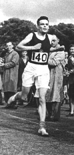
Figure: Alan Turing, in 1946 he was only 11 minutes slower than the winner of the 1948 games. Would he have won a hypothetical games held in 1946? Source: Alan Turing Internet Scrapbook.

If we had to summarise the objectives of machine learning in one word, a very good candidate for that word would be generalization. What is generalization? From a human perspective it might be summarised as the ability to take lessons learned in one domain and apply them to another domain. If we accept the definition given in the first session for machine learning, \[ \text{data} + \text{model} \stackrel{\text{compute}}{\rightarrow} \text{prediction} \] then we see that without a model we can’t generalise: we only have data. Data is fine for answering very specific questions, like “Who won the Olympic Marathon in 2012?”, because we have that answer stored, however, we are not given the answer to many other questions. For example, Alan Turing was a formidable marathon runner, in 1946 he ran a time 2 hours 46 minutes (just under four minutes per kilometer, faster than I and most of the other Endcliffe Park Run runners can do 5 km). What is the probability he would have won an Olympics if one had been held in 1946?

To answer this question we need to generalize, but before we formalize the concept of generalization let’s introduce some formal representation of what it means to generalize in machine learning.

Gaussian Process Fit

Our first objective will be to perform a Gaussian process fit to the data, we’ll do this using the GPy software.

import GPy

m_full = GPy.models.GPRegression(x,yhat)
_ = m_full.optimize() # Optimize parameters of covariance function

The first command sets up the model, then m_full.optimize() optimizes the parameters of the covariance function and the noise level of the model. Once the fit is complete, we’ll try creating some test points, and computing the output of the GP model in terms of the mean and standard deviation of the posterior functions between 1870 and 2030. We plot the mean function and the standard deviation at 200 locations. We can obtain the predictions using y_mean, y_var = m_full.predict(xt)

xt = np.linspace(1870,2030,200)[:,np.newaxis]
yt_mean, yt_var = m_full.predict(xt)
yt_sd=np.sqrt(yt_var)

Now we plot the results using the helper function in mlai.plot.

Figure: Gaussian process fit to the Olympic Marathon data. The error bars are too large, perhaps due to the outlier from 1904.

Fit Quality

In the fit we see that the error bars (coming mainly from the noise variance) are quite large. This is likely due to the outlier point in 1904, ignoring that point we can see that a tighter fit is obtained. To see this make a version of the model, m_clean, where that point is removed.

x_clean=np.vstack((x[0:2, :], x[3:, :]))
y_clean=np.vstack((yhat[0:2, :], yhat[3:, :]))

m_clean = GPy.models.GPRegression(x_clean,y_clean)
_ = m_clean.optimize()

Deep GP Fit

Let’s see if a deep Gaussian process can help here. We will construct a deep Gaussian process with one hidden layer (i.e. one Gaussian process feeding into another).

Build a Deep GP with an additional hidden layer (one dimensional) to fit the model.

import GPy
import deepgp

hidden = 1
m = deepgp.DeepGP([y.shape[1],hidden,x.shape[1]],Y=yhat, X=x, inits=['PCA','PCA'], 
                  kernels=[GPy.kern.RBF(hidden,ARD=True),
                           GPy.kern.RBF(x.shape[1],ARD=True)], # the kernels for each layer
                  num_inducing=50, back_constraint=False)

# Call the initalization
m.initialize()

Now optimize the model.

for layer in m.layers:
    layer.likelihood.variance.constrain_positive(warning=False)
m.optimize(messages=True,max_iters=10000)

m.staged_optimize(messages=(True,True,True))

Olympic Marathon Data Deep GP

Figure: Deep GP fit to the Olympic marathon data. Error bars now change as the prediction evolves.

Olympic Marathon Data Deep GP

Figure: Point samples run through the deep Gaussian process show the distribution of output locations.

Fitted GP for each layer

Now we explore the GPs the model has used to fit each layer. First of all, we look at the hidden layer.

Figure: The mapping from input to the latent layer is broadly, with some flattening as time goes on. Variance is high across the input range.

Figure: The mapping from the latent layer to the output layer.

Olympic Marathon Pinball Plot

Figure: A pinball plot shows the movement of the ‘ball’ as it passes through each layer of the Gaussian processes. Mean directions of movement are shown by lines. Shading gives one standard deviation of movement position. At each layer, the uncertainty is reset. The overal uncertainty is the cumulative uncertainty from all the layers. There is some grouping of later points towards the right in the first layer, which also injects a large amount of uncertainty. Due to flattening of the curve in the second layer towards the right the uncertainty is reduced in final output.

The pinball plot shows the flow of any input ball through the deep Gaussian process. In a pinball plot a series of vertical parallel lines would indicate a purely linear function. For the olypmic marathon data we can see the first layer begins to shift from input towards the right. Note it also does so with some uncertainty (indicated by the shaded backgrounds). The second layer has less uncertainty, but bunches the inputs more strongly to the right. This input layer of uncertainty, followed by a layer that pushes inputs to the right is what gives the heteroschedastic noise.

Deep Emulation

Figure: A potential path of models in the emulation of a simulation system.

As a solution we can use of emulators. When constructing an ML system, software engineers, ML engineers, economists and operations researchers are explicitly defining relationships between variables of interest in the system. That implicitly defines a joint distribution, \(p(\mathbf{ y}^*, \mathbf{ y})\). In a decomposable system any sub-component may be defined as \(p(\mathbf{ y}_\mathbf{i}|\mathbf{ y}_\mathbf{j})\) where \(\mathbf{ y}_\mathbf{i}\) and \(\mathbf{ y}_\mathbf{j}\) represent sub-sets of the full set of variables \(\left\{\mathbf{ y}^*, \mathbf{ y}\right\}\). In those cases where the relationship is deterministic, the probability density would collapse to a vector-valued deterministic function, \(\mathbf{ f}_\mathbf{i}\left(\mathbf{ y}_\mathbf{j}\right)\).

Inter-variable relationships could be defined by, for example a neural network (machine learning), an integer program (operational research), or a simulation (supply chain). This makes probabilistic inference in this joint density for real world systems is either very hard or impossible.

Emulation is a form of meta-modelling: we construct a model of the model. We can define the joint density of an emulator as \(s(\mathbf{ y}*, \mathbf{ y})\), but if this probability density is to be an accurate representation of our system, it is likely to be prohibitively complex. Current practice is to design an emulator to deal with a specific question. This is done by fitting an ML model to a simulation from the the appropriate conditional distribution, \(p(\mathbf{ y}_\mathbf{i}|\mathbf{ y}_\mathbf{j})\), which is intractable. The emulator provides an approximated answer of the form \(s(\mathbf{ y}_\mathbf{i}|\mathbf{ y}_\mathbf{j})\). Critically, an emulator should incorporate its uncertainty about its approximation. So the emulator answer will be less certain than direct access to the conditional \(p(\mathbf{ y}_i|\mathbf{ y}_j)\), but it may be sufficiently confident to act upon. Careful design of emulators to answer a given question leads to efficient diagnostics and understanding of the system. But in a complex interacting system an exponentially increasing number of questions can be asked. This calls for a system of automated construction of emulators which selects the right structure and redeploys the emulator as necessary. Rapid redeployment of emulators could exploit pre-existing emulators through transfer learning.

Automatically deploying these families of emulators for full system understanding is highly ambitious. It requires advances in engineering infrastructure, emulation, and Bayesian optimization. However, the intermediate steps of developing this architecture also allow for automated monitoring of system accuracy and fairness. This facilitates AutoML on a component-wise basis which we can see as a simple implementation of AutoAI. The proposal is structured so that despite its technical ambition there is a smooth ramp of benefits to be derived across the program of work.

In Applied Mathematics, the field studying these techniques is known as uncertainty quantification. The new challenge is the automation of emulator creation on demand to answer questions of interest and facilitate the system design, i.e. AutoAI through BSO.

At design stage, any AI task could be decomposed in multiple ways. Bayesian system optimization will assist both in determining the large-scale system design through exploring different decompositions and in refinement of the deployed system.

So far, most work on emulators has focused on emulating a single component. Automated deployment and maintenance of ML systems requires networks of emulators that can be deployed and redeployed on demand depending on the question of interest. Therefore, the technical innovations we require are in the mathematical composition of emulator models (Damianou and Lawrence, 2013; Paris Perdikaris et al., 2017). Different chains of emulators will need to be rapidly composed to make predictions of downstream performance. This requires rapid retraining of emulators and propagation of uncertainty through the emulation pipeline a process we call deep emulation.

This structural learning allows us to associate data with the relevant layer of the model, rather than merely on the leaf nodes of the output model. When deploying the deep Gaussian process as an emulator, this allows for the possibility of learning the structure of the different component parts of the underlying system. This should aid the user in determining the ideal system decomposition.

Figure: A potential path of models in a machine learning system.

Figure: A potential path of models in the emulation of a simulation system.

Figure: A potential path of models in the emulation of a simulation system.

Brief Reflection

In this module, we have been introducing various aspects of surrogate modelling. We’ve already seen in the sensitivity analysis section, how we used experimental design to make our acquisition of data for the Catapult simulator more efficient. To round of the taught session of the course, we’ll also combine ideas from Bayesian optimization, with an emulator built through experimental design.

The task is a classic example from reinforcement learning, known as the ‘Mountain Car’. The idea is to drive an underpowered car up a hill. The car doesn’t have the ability to accelerate hard enough, but it can build momentum by oscillating up and down a hill to get to the target.

We provide some wrappers of the OpenAI Gym version of the mountain car simulation in a python file. We will use this example to combine various ideas from surrogate modelling to solve the problem.

Figure: The mountain car example contains a simulation of a car’s dynamics within the wider simulation of the mountain. The simulation of the car is called as a subroutine many times by the wider simulation of the mountain. We can choose to build a surrogate model of the car, and work with a modified mountain simulation where the emulator is called instead of the car’s simulation directly.

Mountain Car Simulator

To illustrate the above mentioned concepts we use the mountain car simulator. This simulator is widely used in machine learning to test reinforcement learning algorithms. The goal is to define a control policy on a car whose objective is to climb a mountain. Graphically, the problem looks as follows:

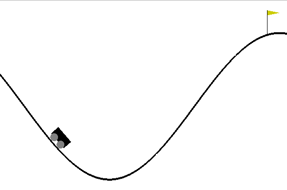
Figure: The mountain car simulation from the Open AI gym.

The goal is to define a sequence of actions (push the car right or left with certain intensity) to make the car reach the flag after a number \(T\) of time steps.

At each time step \(t\), the car is characterized by a vector \(\mathbf{ x}_{t} = (p_t,v_t)\) of states which are respectively the the position and velocity of the car at time \(t\). For a sequence of states (an episode), the dynamics of the car is given by

\[ \mathbf{ x}_{t+1} = f(\mathbf{ x}_{t},\textbf{u}_{t}) \]

where \(\textbf{u}_{t}\) is the value of an action force, which in this example corresponds to push car to the left (negative value) or to the right (positive value). The actions across a full episode are represented in a policy \(\textbf{u}_{t} = \pi(\mathbf{ x}_{t},\theta)\) that acts according to the current state of the car and some parameters \(\theta\). In the following examples we will assume that the policy is linear which allows us to write \(\pi(\mathbf{ x}_{t},\theta)\) as

Mountain Car Set Up

To run the mountain car example we need to install a python file that we’ll download.

import urllib.request

urllib.request.urlretrieve('https://raw.githubusercontent.com/lawrennd/talks/gh-pages/mountain_car.py','mountain_car.py')

And to render the environment, the pyglet library.

%pip install pyglet

\[ \pi(\mathbf{ x},\theta)= \theta_0 + \theta_p p + \theta_vv. \] For \(t=1,\dots,T\) now given some initial state \(\mathbf{ x}_{0}\) and some some values of each \(\textbf{u}_{t}\), we can simulate the full dynamics of the car for a full episode using Gym. The values of \(\textbf{u}_{t}\) are fully determined by the parameters of the linear controller.

After each episode of length \(T\) is complete, a reward function \(R_{T}(\theta)\) is computed. In the mountain car example, the reward is computed as 100 for reaching the target of the hill on the right hand side, minus the squared sum of actions (a real negative to push to the left and a real positive to push to the right) from start to goal. Note that our reward depends on \(\theta\) as we make it dependent on the parameters of the linear controller.

Emulate the Mountain Car

%pip install gym

import gym

env = gym.make('MountainCarContinuous-v0')

Our goal in this section is to find the parameters \(\theta\) of the linear controller such that

\[ \theta^* = arg \max_{\theta} R_T(\theta). \]

In this section, we directly use Bayesian optimization to solve this problem. We will use EmuKit so we first define the objective function.

import mountain_car as mc
import numpy as np

For each set of parameter values of the linear controller we can run an episode of the simulator (that we fix to have a horizon of \(T=500\)) to generate the reward. Using as input the parameters of the controller and as outputs the rewards we can build a Gaussian process emulator of the reward.

We start defining the input space, which is three-dimensional:

from emukit.core import ContinuousParameter, ParameterSpace

position_domain = [-1.2, +1]
velocity_domain = [-1/0.07, +1/0.07]
constant_domain = [-1, +1]

space = ParameterSpace(
          [ContinuousParameter('position_parameter', *position_domain), 
           ContinuousParameter('velocity_parameter', *velocity_domain),
           ContinuousParameter('constant', *constant_domain)])

To initalize the model we start sampling some initial points for the linear controller randomly.

from emukit.core.initial_designs import RandomDesign

design = RandomDesign(space)
n_initial_points = 25
initial_design = design.get_samples(n_initial_points)

Now run the simulation 25 times across our initial design.

y = target_function(initial_design)

Before we start any optimization, lets have a look to the behaviour of the car with the first of these initial points that we have selected randomly.

import numpy as np

This won’t render in Google colab, but should work in a regular Jupyter notebook if pyglet is installed. Details on rendering in colab are given in answer to this stackoverflow question https://stackoverflow.com/questions/50107530/how-to-render-openai-gym-in-google-colab.

random_controller = initial_design[0,:]
_, _, _, frames = mc.run_simulation(env, np.atleast_2d(random_controller), render=True)
anim=mc.animate_frames(frames, 'Random linear controller')

Figure: Random linear controller for the Mountain car. It fails to move the car to the top of the mountain.

As we can see the random linear controller does not manage to push the car to the top of the mountain. Now, let’s optimize the regret using Bayesian optimization and the emulator for the reward. We try 50 new parameters chosen by the expected improvement acquisition function.

First, we initizialize a Gaussian process emulator.

import GPy

kern = GPy.kern.RBF(3)
model_gpy = GPy.models.GPRegression(initial_design, y, kern, noise_var=1e-10)

from emukit.model_wrappers.gpy_model_wrappers import GPyModelWrapper

model_emukit = GPyModelWrapper(model_gpy, n_restarts=5)
model_emukit.optimize()

In Bayesian optimization an acquisition function is used to balance exploration and exploitation to evaluate new locations close to the optimum of the objective. In this notebook we select the expected improvement (EI). For further details have a look at the review paper of Shahriari et al. (2016).

from emukit.bayesian_optimization.acquisitions import ExpectedImprovement

acquisition = ExpectedImprovement(model_emukit)

from emukit.bayesian_optimization.loops.bayesian_optimization_loop import BayesianOptimizationLoop

bo = BayesianOptimizationLoop(space, model_emukit, acquisition=acquisition)
bo.run_loop(target_function, 50)
results= bo.get_results()

Now we visualize the result for the best controller that we have found with Bayesian optimization.

_, _, _, frames = mc.run_simulation(env, np.atleast_2d(results.minimum_location), render=True)
anim=mc.animate_frames(frames, 'Best controller after 50 iterations of Bayesian optimization')

Figure: Mountain car simulator trained using Bayesian optimization and the simulator of the dynamics. Fifty iterations of Bayesian optimization are used to optimize the controler.

The car can now make it to the top of the mountain! Emulating the reward function and using expected improvement acquisition helped us to find a linear controller that solves the problem.

Data Efficient Emulation

In the previous section we solved the mountain car problem by directly emulating the reward but no considerations about the dynamics \[ \mathbf{ x}_{t+1} =g(\mathbf{ x}_{t},\textbf{u}_{t}) \] of the system were made.

We ran the simulator 25 times in the initial design, and 50 times in our Bayesian optimization loop. That required us to call the dynamics simulation \(500\times 75 =37,500\) times, because each simulation of the car used 500 steps. In this section we will show how it is possible to reduce this number by building an emulator for \(g(\cdot)\) that can later be used to directly optimize the control.

The inputs of the model for the dynamics are the velocity, the position and the value of the control so create this space accordingly.

import gym

env = gym.make('MountainCarContinuous-v0')

from emukit.core import ContinuousParameter, ParameterSpace

position_dynamics_domain = [-1.2, +0.6]
velocity_dynamics_domain = [-0.07, +0.07]
action_dynamics_domain = [-1, +1]

space_dynamics = ParameterSpace(
          [ContinuousParameter('position_dynamics_parameter', *position_dynamics_domain), 
           ContinuousParameter('velocity_dynamics_parameter', *velocity_dynamics_domain),
           ContinuousParameter('action_dynamics_parameter', *action_dynamics_domain)])

Next, we sample some input parameters and use the simulator to compute the outputs. Note that in this case we are not running the full episodes, we are just using the simulator to compute \(\mathbf{ x}_{t+1}\) given \(\mathbf{ x}_{t}\) and \(\textbf{u}_{t}\).

from emukit.core.initial_designs import RandomDesign

design_dynamics = RandomDesign(space_dynamics)
n_initial_points = 500
initial_design_dynamics = design_dynamics.get_samples(n_initial_points)

import numpy as np
import mountain_car as mc

### --- Simulation of the (normalized) outputs
y_dynamics = np.zeros((initial_design_dynamics.shape[0], 2))
for i in range(initial_design_dynamics.shape[0]):
    y_dynamics[i, :] = mc.simulation(initial_design_dynamics[i, :])

# Normalize the data from the simulation
y_dynamics_normalisation = np.std(y_dynamics, axis=0)
y_dynamics_normalised = y_dynamics/y_dynamics_normalisation

The outputs are the velocity and the position. Our model will capture the change in position and velocity on time. That is, we will model

\[ \Delta v_{t+1} = v_{t+1} - v_{t} \]

\[ \Delta x_{t+1} = p_{t+1} - p_{t} \]

with Gaussian processes with prior mean \(v_{t}\) and \(p_{t}\) respectively. As a covariance function, we use Matern52. We need therefore two models to capture the full dynamics of the system.

import GPy

kern_position = GPy.kern.Matern52(3)
position_model_gpy = GPy.models.GPRegression(initial_design_dynamics, y_dynamics[:, 0:1], kern_position, noise_var=1e-10)

kern_velocity = GPy.kern.Matern52(3)
velocity_model_gpy = GPy.models.GPRegression(initial_design_dynamics, y_dynamics[:, 1:2], kern_velocity, noise_var=1e-10)

from emukit.model_wrappers.gpy_model_wrappers import GPyModelWrapper

position_model_emukit = GPyModelWrapper(position_model_gpy, n_restarts=5)
velocity_model_emukit = GPyModelWrapper(velocity_model_gpy, n_restarts=5)

In general, we might use much smarter strategies to design our emulation of the simulator. For example, we could use the variance of the predictive distributions of the models to collect points using uncertainty sampling, which will give us a better coverage of the space. For simplicity, we move ahead with the 500 randomly selected points.

Now that we have a data set, we can update the emulators for the location and the velocity.

position_model_emukit.optimize()
velocity_model_emukit.optimize()

We can now have a look to how the emulator and the simulator match. First, we show a contour plot of the car acceleration for each pair of can position and velocity. You can use the bar bellow to play with the values of the controller to compare the emulator and the simulator.

We can see how the emulator is doing a fairly good job approximating the simulator. On the edges, however, it struggles to captures the dynamics of the simulator.

Given some input parameters of the linear controlling, how do the dynamics of the emulator and simulator match? In the following figure we show the position and velocity of the car for the 500 time-steps of an episode in which the parameters of the linear controller have been fixed beforehand. The value of the input control is also shown.

# change the values of the linear controller to observe the trajectories.
controller_gains = np.atleast_2d([0, .6, 1])  

Figure: Comparison between the mountain car simulator and the emulator.

We now make explicit use of the emulator, using it to replace the simulator and optimize the linear controller. Note that in this optimization, we don’t need to query the simulator anymore as we can reproduce the full dynamics of an episode using the emulator. For illustrative purposes, in this example we fix the initial location of the car.

We define the objective reward function in terms of the simulator.

### --- Optimize control parameters with emulator
car_initial_location = np.asarray([-0.58912799, 0])

And as before, we use Bayesian optimization to find the best possible linear controller.

The design space is the three continuous variables that make up the linear controller.

position_domain = [-1.2, +1]
velocity_domain = [-1/0.07, +1/0.07]
constant_domain = [-1, +1]

space = ParameterSpace(
          [ContinuousParameter('position_parameter', *position_domain), 
           ContinuousParameter('velocity_parameter', *velocity_domain),
           ContinuousParameter('constant', *constant_domain)])

from emukit.core.initial_designs import RandomDesign

design = RandomDesign(space)
n_initial_points = 25
initial_design = design.get_samples(n_initial_points)

Now run the simulation 25 times across our initial design.

y = target_function_emulator(initial_design)

Now we set up the surrogate model for the Bayesian optimization loop.

import GPy

kern = GPy.kern.RBF(3)
model_dynamics_emulated_gpy = GPy.models.GPRegression(initial_design, y, kern, noise_var=1e-10)

from emukit.model_wrappers.gpy_model_wrappers import GPyModelWrapper

model_dynamics_emulated_emukit = GPyModelWrapper(model_dynamics_emulated_gpy, n_restarts=5)
model_dynamics_emulated_emukit.optimize()

We set the acquisition function to be expected improvement.

from emukit.bayesian_optimization.acquisitions import ExpectedImprovement

acquisition = ExpectedImprovement(model_emukit)

And we set up the main loop for the Bayesian optimization.

from emukit.bayesian_optimization.loops.bayesian_optimization_loop import BayesianOptimizationLoop

bo = BayesianOptimizationLoop(space, model_dynamics_emulated_emukit, acquisition=acquisition)
bo.run_loop(target_function_emulator, 50)
results = bo.get_results()

_, _, _, frames = mc.run_simulation(env, np.atleast_2d(results.minimum_location), render=True)
anim=mc.animate_frames(frames, 'Best controller using the emulator of the dynamics')

from IPython.core.display import HTML

Figure: Mountain car controller learnt through emulation. Here 500 calls to the simulator are used to fit the controller rather than 37,500 calls to the simulator required in the standard learning.

And the problem is again solved, but in this case, we have replaced the simulator of the car dynamics by a Gaussian process emulator that we learned by calling the dynamics simulator only 500 times. Compared to the 37,500 calls that we needed when applying Bayesian optimization directly on the simulator this is a significant improvement. Of course, in practice the car dynamics are very simple for this example.

Mountain Car: Multi-Fidelity Emulation

In some scenarios we have simulators of the same environment that have different fidelities, that is that reflect with different level of accuracy the dynamics of the real world. Running simulations of the different fidelities also have a different cost: high-fidelity simulations are typically more expensive the low-fidelity. If we have access to these simulators, we can combine high and low-fidelity simulations under the same model.

So, let’s assume that we have two simulators of the mountain car dynamics, one of high fidelity (the one we have used) and another one of low fidelity. The traditional approach to this form of multi-fidelity emulation is to assume that \[ f_i\left(\mathbf{ x}\right) = \rho f_{i-1}\left(\mathbf{ x}\right) + \delta_i\left(\mathbf{ x}\right), \] where \(f_{i-1}\left(\mathbf{ x}\right)\) is a low-fidelity simulation of the problem of interest and \(f_i\left(\mathbf{ x}\right)\) is a higher fidelity simulation. The function \(\delta_i\left(\mathbf{ x}\right)\) represents the difference between the lower and higher fidelity simulation, which is considered additive. The additive form of this covariance means that if \(f_{0}\left(\mathbf{ x}\right)\) and \(\left\{\delta_i\left(\mathbf{ x}\right)\right\}_{i=1}^m\) are all Gaussian processes, then the process over all fidelities of simulation will be a joint Gaussian process.

But with deep Gaussian processes we can consider the form \[ f_i\left(\mathbf{ x}\right) = g_{i}\left(f_{i-1}\left(\mathbf{ x}\right)\right) + \delta_i\left(\mathbf{ x}\right), \] where the low fidelity representation is nonlinearly transformed by \(g(\cdot)\) before use in the process. This is the approach taken in P. Perdikaris et al. (2017). But once we accept that these models can be composed, a highly flexible framework can emerge. A key point is that the data enters the model at different levels and represents different aspects. For example, these correspond to the two fidelities of the mountain car simulator.

We start by sampling both at 250 random input locations.

import gym

env = gym.make('MountainCarContinuous-v0')

from emukit.core import ContinuousParameter, ParameterSpace

position_dynamics_domain = [-1.2, +0.6]
velocity_dynamics_domain = [-0.07, +0.07]
action_dynamics_domain = [-1, +1]

space_dynamics = ParameterSpace(
          [ContinuousParameter('position_dynamics_parameter', *position_dynamics_domain), 
           ContinuousParameter('velocity_dynamics_parameter', *velocity_dynamics_domain),
           ContinuousParameter('action_dynamics_parameter', *action_dynamics_domain)])

Next, we evaluate the high and low fidelity simualtors at those locations.

import numpy as np
import mountain_car as mc

n_points = 250
d_position_hf = np.zeros((n_points, 1))
d_velocity_hf = np.zeros((n_points, 1))
d_position_lf = np.zeros((n_points, 1))
d_velocity_lf = np.zeros((n_points, 1))

# --- Collect high fidelity points
for i in range(0, n_points):
    d_position_hf[i], d_velocity_hf[i] = mc.simulation(x_random[i, :])

# --- Collect low fidelity points  
for i in range(0, n_points):
    d_position_lf[i], d_velocity_lf[i] = mc.low_cost_simulation(x_random[i, :])

Prime Air

One project where the components of machine learning and the physical world come together is Amazon’s Prime Air drone delivery system.

Automating the process of moving physical goods through autonomous vehicles completes the loop between the ‘bits’ and the ‘atoms’. In other words, the information and the ‘stuff’. The idea of the drone is to complete a component of package delivery, the notion of last mile movement of goods, but in a fully autonomous way.

Figure: An actual ‘Santa’s sleigh’. Amazon’s prototype delivery drone. Machine learning algorithms are used across various systems including sensing (computer vision for detection of wires, people, dogs etc) and piloting. The technology is necessarily a combination of old and new ideas. The transition from vertical to horizontal flight is vital for efficiency and uses sophisticated machine learning to achieve.

As Jeff Wilke (who was CEO of Amazon Retail at the time) announced in June 2019 the technology is ready, but still needs operationalization including e.g. regulatory approval.

Figure: Jeff Wilke (CEO Amazon Consumer) announcing the new drone at the Amazon 2019 re:MARS event alongside the scale of the Amazon supply chain.

When we announced earlier this year that we were evolving our Prime two-day shipping offer in the U.S. to a one-day program, the response was terrific. But we know customers are always looking for something better, more convenient, and there may be times when one-day delivery may not be the right choice. Can we deliver packages to customers even faster? We think the answer is yes, and one way we’re pursuing that goal is by pioneering autonomous drone technology.

Today at Amazon’s re:MARS Conference (Machine Learning, Automation, Robotics and Space) in Las Vegas, we unveiled our latest Prime Air drone design. We’ve been hard at work building fully electric drones that can fly up to 15 miles and deliver packages under five pounds to customers in less than 30 minutes. And, with the help of our world-class fulfillment and delivery network, we expect to scale Prime Air both quickly and efficiently, delivering packages via drone to customers within months.

The 15 miles in less than 30 minutes implies air speed velocities of around 50 kilometers per hour.

Our newest drone design includes advances in efficiency, stability and, most importantly, in safety. It is also unique, and it advances the state of the art. How so? First, it’s a hybrid design. It can do vertical takeoffs and landings – like a helicopter. And it’s efficient and aerodynamic—like an airplane. It also easily transitions between these two modes—from vertical-mode to airplane mode, and back to vertical mode.

It’s fully shrouded for safety. The shrouds are also the wings, which makes it efficient in flight.

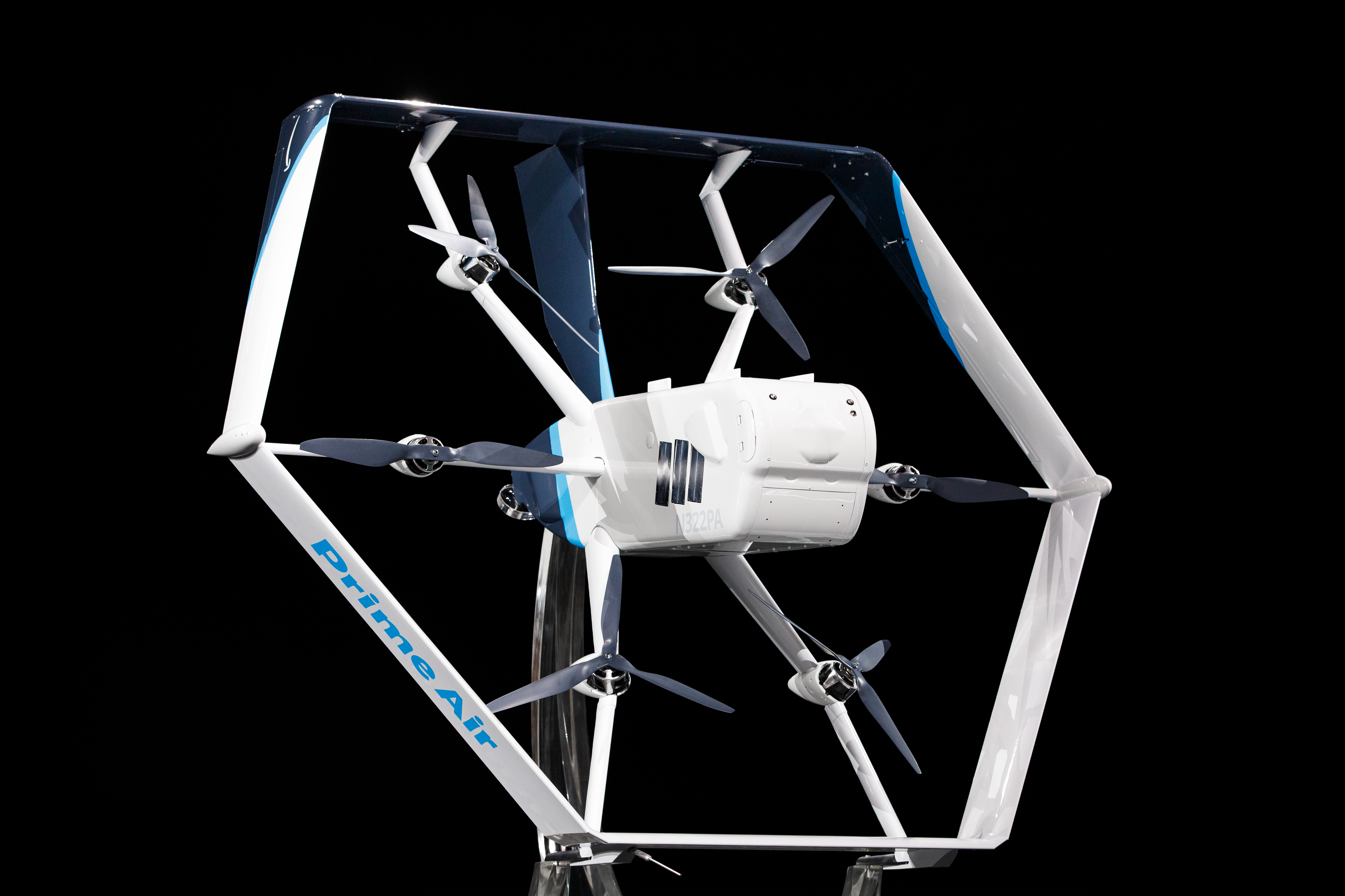
Figure: Picture of the drone from Amazon Re-MARS event in 2019.

Our drones need to be able to identify static and moving objects coming from any direction. We employ diverse sensors and advanced algorithms, such as multi-view stereo vision, to detect static objects like a chimney. To detect moving objects, like a paraglider or helicopter, we use proprietary computer-vision and machine learning algorithms.

A customer’s yard may have clotheslines, telephone wires, or electrical wires. Wire detection is one of the hardest challenges for low-altitude flights. Through the use of computer-vision techniques we’ve invented, our drones can recognize and avoid wires as they descend into, and ascend out of, a customer’s yard.

Thanks!

For more information on these subjects and more you might want to check the following resources.

• twitter: @lawrennd
• podcast: The Talking Machines
• newspaper: Guardian Profile Page
• blog: http://inverseprobability.com

References