Week 5: Sensitivity Analysis

[jupyter][google colab][reveal]

Neil D. Lawrence

Abstract:

This week we introduce sensitivity analysis through Emukit, showing how Emukit can deliver Sobol indices for understanding how the output of the system is affected by different inputs.

Setup

notutils

This small package is a helper package for various notebook utilities used below.

The software can be installed using

%pip install notutils

from the command prompt where you can access your python installation.

The code is also available on GitHub: https://github.com/lawrennd/notutils

Once notutils is installed, it can be imported in the usual manner.

import notutils

pods

In Sheffield we created a suite of software tools for ‘Open Data Science’. Open data science is an approach to sharing code, models and data that should make it easier for companies, health professionals and scientists to gain access to data science techniques.

You can also check this blog post on Open Data Science.

The software can be installed using

%pip install pods

from the command prompt where you can access your python installation.

The code is also available on GitHub: https://github.com/lawrennd/ods

Once pods is installed, it can be imported in the usual manner.

import pods

mlai

The mlai software is a suite of helper functions for teaching and demonstrating machine learning algorithms. It was first used in the Machine Learning and Adaptive Intelligence course in Sheffield in 2013.

The software can be installed using

%pip install mlai

from the command prompt where you can access your python installation.

The code is also available on GitHub: https://github.com/lawrennd/mlai

Once mlai is installed, it can be imported in the usual manner.

import mlai

%pip install gpy

%pip install pyDOE

%pip install emukit

Emukit Sensitivity Analysis

This introduction is based on Introduction to Global Sensitivity Analysis with Emukit written by Mark Pullin, Javier Gonzalez, Juan Emmanuel Johnson and Andrei Paleyes. Some references include (Kennedy and O’Hagan, 2000; Saltelli et al., 2010, 2008, 2004; Sobol, 2001, 1990)

A possible definition of sensitivity analysis is the following: The study of how uncertainty in the output of a model (numerical or otherwise) can be apportioned to different sources of uncertainty in the model input (Saltelli et al., 2004). A related practice is ‘uncertainty analysis’, which focuses rather on quantifying uncertainty in model output. Ideally, uncertainty and sensitivity analyses should be run in tandem, with uncertainty analysis preceding in current practice.

In Chapter 1 of Saltelli et al. (2008)

import numpy as np
import matplotlib.pyplot as plt

from matplotlib import colors as mcolors
from matplotlib import cm

%pip install pyDOE

import mlai
import mlai.plot as plot

Sensitivity analysis is a statistical technique widely used to test the reliability of real systems. Imagine a simulator of taxis picking up customers in a city like the one showed in the Emukit playground. The profit of the taxi company depends on factors like the number of taxis on the road and the price per trip. In this example, a global sensitivity analysis of the simulator could be useful to decompose the variance of the profit in a way that can be assigned to the input variables of the simulator.

There are different ways of doing a sensitivity analysis of the variables of a simulator. In this notebook we will start with an approach based on Monte Carlo sampling that is useful when evaluating the simulator is cheap. If evaluating the simulator is expensive, emulators can then be used to speed up computations. We will show this in the last part of the notebook. Next, we start with a few formal definitions and literature review so we can understand the basics of Sensitivity Analysis and how it can be performed with Emukit.

Local Sensitivity

Given any function, \(g(\cdot)\), we might be interested in how sensitive that function is to variations in its input space. One route to determining this is to compute the partial derivatives of that function with respect to its inputs, \[ \frac{\partial}{\partial x_i} g(\mathbf{ x}). \] The matrix of all these partial derivatives is known as the Jacobian.

These types of local sensitivity analysis can be used for determining the effect of changing an input variable around an operating point. But they don’t give us an understanding of the response of the target function to variations in the input across the domain of inputs. For this, we need to look to global sensitivity analysis.

Global Sensitivity Analysis

In global sensitivity analysis, rather than looking around a single operating point, we’re interested in the overall sensitivity of a function to its inputs, or combinations of inputs, across its entire domain. The key tool in determining this sensitivity is known as the ANOVA decomposition, or the Hoeffding-Sobol decomposition.

For global sensitivity analysis, we need to make an assumption about how inputs are going to vary to create different values of the function. The fundamental object we’re interested in is the total variance of the function, \[ \text{var}\left(g(\mathbf{ x})\right) = \left\langle g(\mathbf{ x})^2 \right\rangle _{p(\mathbf{ x})} - \left\langle g(\mathbf{ x}) \right\rangle _{p(\mathbf{ x})}^2, \] where \[ \left\langle h(\mathbf{ x}) \right\rangle _{p(\mathbf{ x})} = \int_\mathbf{ x}h(\mathbf{ x}) p(\mathbf{ x}) \text{d}\mathbf{ x} \] is the expectation of the function \(h(\mathbf{ x})\) under the density \(p(\mathbf{ x})\), which represents the probability distribution of inputs we’re interested in.

The total variance of the function gives us the overall variation of the function across the domain of inputs, as represented by the probability density, \(p(\mathbf{ x})\). Normally, we perform analysis by assuming that, \[ p(\mathbf{ x}) = \prod_{i=1}^pp(x_i) \] and that each \(p(x_i)\) is uniformly distributed across its input domain. Assuming we scale the input domain down to the interval \([0, 1]\), that gives us \[ x_i \sim \mathcal{U}\left(0,1\right). \]

Hoeffding-Sobol Decomposition

The Hoeffding-Sobol, or ANOVA, decomposition of a function allows us to write it as, \[ \begin{align*} g(\mathbf{ x}) = & g_0 + \sum_{i=1}^pg_i(x_i) + \sum_{i<j}^{p} g_{ij}(x_i,x_j) + \cdots \\ & + g_{1,2,\dots,p}(x_1,x_2,\dots,x_p), \end{align*} \] where \[ g_0 = \left\langle g(\mathbf{ x}) \right\rangle _{p(\mathbf{ x})} \] and \[ g_i(x_i) = \left\langle g(\mathbf{ x}) \right\rangle _{p(\mathbf{ x}_{\sim i})} - g_0, \] where we’re using the notation \(p(\mathbf{ x}_{\sim i})\) to represent the input distribution with the \(i\)th variable marginalised, \[ p(\mathbf{ x}_{\sim i}) = \int p(\mathbf{ x}) \text{d}x_i \] Higher order terms in the decomposition represent interactions between inputs, \[ g_{i,j}(x_i, x_j) = \left\langle g(\mathbf{ x}) \right\rangle _{p(\mathbf{ x}_{\sim i,j})} - g_i(x_i) - g_j(x_j) - g_0 \] and similar expressions can be written for higher order terms up to \(g_{1,2,\dots,p}(\mathbf{ x})\).

Note that to compute each of these individual terms, you need to first compute the low order terms, and then compute the high order terms. This can be problematic when \(p\) is large.

We’re interested in the variance of the function \(g\), so implicitly we’re assuming that the square of this function is integrable across its domain, i.e., we’re assuming that \(\left\langle g(\mathbf{ x})^2 \right\rangle _{p(\mathbf{ x})}\) exists and is finite.

The Sobol decomposition has some important properties, in particular, its components are orthogonal, so this means that when we substitute it in to the variance, we have, \[ \begin{align*} \text{var}(g) = & \left\langle g(\mathbf{ x})^2 \right\rangle _{p(\mathbf{ x})} - \left\langle g(\mathbf{ x}) \right\rangle _{p(\mathbf{ x})}^2 \\ = & \left\langle g(\mathbf{ x})^2 \right\rangle _{p(\mathbf{ x})} - g_0^2\\ = & \sum_{i=1}^p\text{var}\left(g_i(x_i)\right) + \sum_{i<j}^{p} \text{var}\left(g_{ij}(x_i,x_j)\right) + \cdots \\ & + \text{var}\left(g_{1,2,\dots,p}(x_1,x_2,\dots,x_p)\right). \end{align*} \] So, this decomposition gives us a decomposition of the function in terms of variances. It’s for this reason that it’s sometimes known as an ANOVA decomposition. ANOVA stands a for analysis of variance. The ANOVA decomposition decomposes the function into additive variance parts that are each stemming from interactions between different inputs.

As is common in various analyses of variance, we can rescale the components with the total variance of the function. These rescaled components are known as Sobol indicies. \[ S_\ell = \frac{\text{var}\left(g(\mathbf{ x}_\ell)\right)}{\text{var}\left(g(\mathbf{ x})\right)}, \] where the \(\ell\) represents the relevent set of indices for the different combinations of inputs.

In practice, for an elegant approach that exploits a particular covariance function structure to perform global sensitivity analysis see Durrande et al. (2013).

Example: the Ishigami function

We illustrate the exact calculation of the Sobol indices with the three-dimensional Ishigami function of (Ishigami and Homma, 1989).

Ishigami Function

The Ishigami function (Ishigami and Homma, 1989) is a well-known test function for uncertainty and sensitivity analysis methods because of its strong nonlinearity and peculiar dependence on \(x_3\). More details of this function can be found in (Sobol and Levitan, 1999).

Mathematically, the form of the Ishigami function is \[ g(\textbf{x}) = \sin(x_1) + a \sin^2(x_2) + b x_3^4 \sin(x_1). \] We will set the parameters to be \(a = 5\) and \(b=0.1\) . The input variables are sampled randomly \(x_i \sim \mathcal{U}\left(-\pi,\pi\right)\).

Next, we create the function object and visualize its shape marginally for each one of its three inputs.

Load the Ishigami function

from emukit.test_functions.sensitivity import Ishigami

ishigami = Ishigami(a=5, b=0.1)
target_function = ishigami.fidelity1

That gives us the target function, next we define the input space for the simulator.

import numpy as np
from emukit.core import ContinuousParameter, ParameterSpace

variable_domain = (-np.pi,np.pi)
           
space = ParameterSpace(
          [ContinuousParameter('x1', *variable_domain), 
           ContinuousParameter('x2', *variable_domain),
           ContinuousParameter('x3', *variable_domain)])

Before moving to any further analysis, we first plot the non-zero components \(g(\mathbf{ x})\). These components are \[ \begin{align*} g_1(x_1) & = \sin(x_1) \\ g_2(x_2) & = a \sin^2 (x_2) \\ g_{13}(x_1,x_3) & = b x_3^4 \sin(x_1) \end{align*} \]

x_grid = np.linspace(*variable_domain,100)
target_simulator = ishigami.fidelity1
f1 = ishigami.f1(x_grid)
f2 = ishigami.f2(x_grid)
F13 = ishigami.f13(np.array([x_grid,x_grid]).T)[:,np.newaxis]

Figure: The non-zero components of the Ishigami function.

Total Variance

The total variance \(\text{var}(y)\) in this example is

print(ishigami.variance_total)

which is the sum of the variance of \(\text{var}\left(g_1(x_1)\right)\), \(\text{var}\left(g_2(x_2)\right)\) and \(\text{var}\left(g_{1,3}(x_{1,3})\right)\)

print(ishigami.variance_x1, ishigami.variance_x2, ishigami.variance_x13)
print(ishigami.variance_x1 + ishigami.variance_x2 + ishigami.variance_x13)

First Order Sobol Indices using Monte Carlo

The first order Sobol indices are a measure of “first order sensitivity” of each input variable. They account for the proportion of variance of \(y\) explained by changing each variable alone while marginalizing over the rest. Recall that the Sobol index of the \(i\)th variable is computed as \[ S_i = \frac{\text{var}\left(g_i(x_i)\right)}{\text{var}\left(g(\mathbf{ x})\right)}. \] This value is standardized using the total variance, so it is possible to account for a fractional contribution of each variable to the total variance of the output.

The Sobol indices for higher order interactions \(S_{i,j}\) are computed similarly. Due to the normalization by the total variance, the the sum of all Sobol indices equals to one.

In most cases we are interested in the first order indices. The Ishigami function has the benefit that these can be computed analytically. In EmuKit you can extract these values with the code.

ishigami.main_effects

But in general, these indices need to be sampled using Monte Carlo or one of the quasi-Monte Carlo methods we’ve seen in the model-free experimental design. Details are given in (Sobol, 2001).

With Emukit, the first-order Sobol indices can be easily computed. We first need to define the space where the target simulator is analyzed.

from emukit.sensitivity.monte_carlo import ModelFreeMonteCarloSensitivity

np.random.seed(10)  # for reproducibility

num_monte_carlo_points = 10000  # Number of MC samples
senstivity_ishigami = ModelFreeMonteCarloSensitivity(target_simulator, space)
main_effects, total_effects, _ = senstivity_ishigami.compute_effects(num_monte_carlo_points = num_monte_carlo_points)
print(main_effects)

We compare the true effects with the Monte Carlo effects in a bar-plot. The total effects are discussed later.

Figure: The non-zero components of the Ishigami function.

Total Effects Using Monte Carlo

Computing high order sensitivity indices can be computationally very demanding in high dimensional scenarios and measuring the total influence of each variable on the variance of the output is infeasible. To solve this issue the total indices are used which account for the contribution to the output variance of \(x_i\) including all variance caused by the variable alone and all its interactions of any order.

The total effect for \(x_i\) is given by: \[ S_{Ti} = \frac{\left\langle \text{var}_{x_i} (y\mid \mathbf{ x}_{\sim i}) \right\rangle _{p(\mathbf{ x}_{\sim i})}}{\text{var}\left(g(\mathbf{ x})\right)} = 1 - \frac{\text{var}_{\mathbf{ x}_{\sim i}} \left\langle y\mid \mathbf{ x}_{\sim i} \right\rangle _{p(\mathbf{ x}_{\sim i})}}{\text{var}\left(g(\mathbf{ x})\right)} \]

Note that the sum of \(S_{Ti}\) is not necessarily one in this case unless the model is additive. In the Ishigami example the value of the total effects is

ishigami.total_effects

As in the previous example, the total effects can be computed with Monte Carlo. In the next plot we show the comparison with the true total effects.

Figure: The total effects from the Ishigami function as computed via Monte Carlo estimate alongside the true total effects for the Ishigami function.

Computing the Sensitivity Indices Using the Output of a Model

In the example used above the Ishigami function is very cheap to evaluate. However, in most real scenarios the functions of interest are expensive, and we need to limit ourselves to a few number of evaluations. Using Monte Carlo methods is infeasible in these scenarios as a large number of samples are typically required to provide good estimates of the Sobol indices.

An alternative in these cases is to use Gaussaian process emulator of the function of interest trained on a few inputs and outputs (Marrel et al., 2009). If the model is properly trained, its mean prediction which is cheap to evaluate, can be used to compute the Monte Carlo estimates of the Sobol indices, the variance from the GP emulator can also be used to assess our uncertainty about the Sobol indices. Let’s see how we can do this in Emukit.

We start by generating 100 samples in the input domain. Note that this a just 1% of the number of samples that we used to compute the Sobol coefficients using Monte Carlo.

from emukit.core.initial_designs import RandomDesign

design = RandomDesign(space)
x = design.get_samples(500)
y = ishigami.fidelity1(x)[:,np.newaxis]

Now, we fit a standard Gaussian process to the samples, and we wrap it as an Emukit model.

from GPy.models import GPRegression
from emukit.model_wrappers import GPyModelWrapper
from emukit.sensitivity.monte_carlo import MonteCarloSensitivity

model_gpy = GPRegression(x,y)
model_emukit = GPyModelWrapper(model_gpy)
model_emukit.optimize()

The final step is to compute the coefficients using the class ModelBasedMonteCarloSensitivity which directly calls the model and uses its predictive mean to compute the Monte Carlo estimates of the Sobol indices. We plot the true estimates, those computed using 10000 direct evaluations of the object using Monte Carlo and those computed using a Gaussian process model trained on 100 evaluations.

num_mc = 10000
senstivity_ishigami_gpbased = MonteCarloSensitivity(model = model_emukit, input_domain = space)
main_effects_gp, total_effects_gp, _ = senstivity_ishigami_gpbased.compute_effects(num_monte_carlo_points = num_mc)

Figure: First order Sobol indices as estimated by Monte Carlo and GP-emulator based Monte Carlo.

Figure: Total effects as estimated by Monte Carlo and GP based Monte Carlo.

We observe some discrepancies with respect to the real value of the Sobol index when using the Gaussian process, but we get a fairly good approximation with a very reduced number of evaluations of the original target function.

Conclusions

The Sobol indices are a tool for explaining the variance of the output of a function as components of the input variables. Monte Carlo is an approach for computing these indices if the function is cheap to evaluate. Other approaches are needed when \(g(\cdot)\) is expensive to compute.

Catapult Simulation

As a worked example we’re going to introduce a catapult simulation written by Nicolas Durrande, https://durrande.shinyapps.io/catapult/.

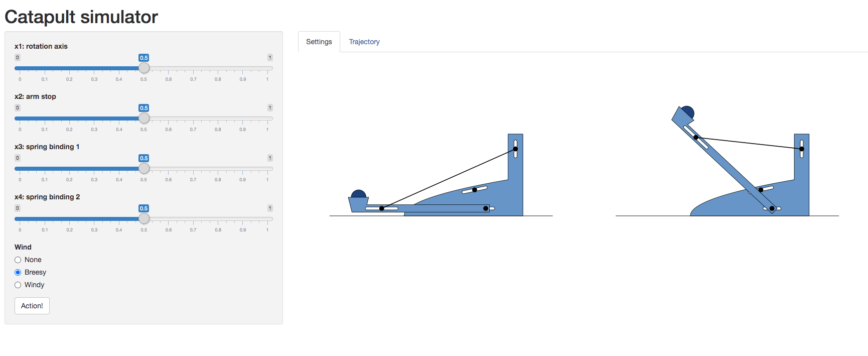
Figure: A catapult simulation for experimenting with surrogate models, kindly provided by Nicolas Durrande

The simulator allows you to set various parameters of the catapult including the axis of rotation, roation_axis, the position of the arm stop, arm_stop, and the location of the two bindings of the catapult’s spring, spring_binding_1 and spring_binding_2.

These parameters are then collated in a vector, \[ \mathbf{ x}_i = \begin{bmatrix} \texttt{rotation_axis} \\ \texttt{arm_stop} \\ \texttt{spring_binding_1} \\ \texttt{spring_binding_2} \end{bmatrix} \]

Having set those parameters, you can run an experiment, by firing the catapult. This will show you how far it goes.

Because you will need to operate the catapult yourself, we’ll create a function to query you about the result of an individual firing.

We can also set the parameter space for the model. Each of these variables is scaled to operate \(\in [0, 1]\).

from emukit.core import ContinuousParameter, ParameterSpace

variable_domain = [0,1]
           
space = ParameterSpace(
          [ContinuousParameter('rotation_axis', *variable_domain), 
           ContinuousParameter('arm_stop', *variable_domain),
           ContinuousParameter('spring_binding_1', *variable_domain),
           ContinuousParameter('spring_binding_2', *variable_domain)])

Before we perform sensitivity analysis, we need to build an emulator of the catapulter, which we do using our experimental design process.

Experimental Design for the Catapult

Now we will build an emulator for the catapult using the experimental design loop.

We’ll start with a small model-free design, we’ll use a random design for initializing our model.

from emukit.core.initial_designs import RandomDesign

design = RandomDesign(space)
x = design.get_samples(5)
y = catapult_distance(x)

from GPy.models import GPRegression
from emukit.model_wrappers import GPyModelWrapper
from emukit.sensitivity.monte_carlo import MonteCarloSensitivity

Set up the GPy model. The variance of the RBF kernel is set to \(150^2\) because that’s roughly the square of the range of the catapult. We set the noise variance to a small value.

model_gpy = GPRegression(x,y)
model_gpy.kern.variance = 150**2
model_gpy.likelihood.variance.fix(1e-5)
display(model_gpy)

Wrap the model for EmuKit.

model_emukit = GPyModelWrapper(model_gpy)
model_emukit.optimize()

display(model_gpy)

Now we set up the model loop. We’ll use integrated variance reduction as the acquisition function for our model-based design loop.

Warning: This loop runs much slower on Google colab than on a local machine.

from emukit.experimental_design.experimental_design_loop import ExperimentalDesignLoop

from emukit.experimental_design.acquisitions import IntegratedVarianceReduction, ModelVariance

integrated_variance = IntegratedVarianceReduction(space=space,
                                                  model=model_emukit)
ed = ExperimentalDesignLoop(space=space, 
                            model=model_emukit, 
                            acquisition = integrated_variance)
ed.run_loop(catapult_distance, 10)

Sensitivity Analysis of a Catapult Simulation

The final step is to compute the coefficients using the class ModelBasedMonteCarloSensitivity which directly calls the model and uses its predictive mean to compute the Monte Carlo estimates of the Sobol indices. We plot the estimates of the Sobol indices computed using a Gaussian process model trained on the observations we’ve acquired.

num_mc = 10000
senstivity = MonteCarloSensitivity(model = model_emukit, input_domain = space)
main_effects_gp, total_effects_gp, _ = senstivity.compute_effects(num_monte_carlo_points = num_mc)

Figure: First Order sobol indices as estimated by GP-emulator based Monte Carlo on the catapult.

Figure: Total effects as estimated by GP based Monte Carlo on the catapult.

Thanks!

For more information on these subjects and more you might want to check the following resources.

• twitter: @lawrennd
• podcast: The Talking Machines
• newspaper: Guardian Profile Page
• blog: http://inverseprobability.com

References