Week 2: Simulation

[jupyter][google colab][reveal]

Neil D. Lawrence

Abstract:

This lecture will introduce the notion of simulation and review the different types of simulation we might use to represent the physical world.

Last lecture Carl Henrik introduced you to some of the challenges of approximate inference. Including the problem of mathematical tractability. Before that he introduced you to a particular form of model, the Gaussian process.

notutils

This small package is a helper package for various notebook utilities used below.

The software can be installed using

%pip install notutils

from the command prompt where you can access your python installation.

The code is also available on GitHub: https://github.com/lawrennd/notutils

Once notutils is installed, it can be imported in the usual manner.

import notutils

mlai

The mlai software is a suite of helper functions for teaching and demonstrating machine learning algorithms. It was first used in the Machine Learning and Adaptive Intelligence course in Sheffield in 2013.

The software can be installed using

%pip install mlai

from the command prompt where you can access your python installation.

The code is also available on GitHub: https://github.com/lawrennd/mlai

Once mlai is installed, it can be imported in the usual manner.

import mlai

Game of Life

John Horton Conway was a mathematician who developed a game known as the Game of Life. He died in April 2020, but since he invented the game, he was in effect ‘god’ for this game. But as we will see, just inventing the rules doesn’t give you omniscience in the game.

The Game of Life is played on a grid of squares, or pixels. Each pixel is either on or off. The game has no players, but a set of simple rules that are followed at each turn the rules are.

Life Rules

John Conway’s game of life is a cellular automaton where the cells obey three very simple rules. The cells live on a rectangular grid, so that each cell has 8 possible neighbors.

loneliness

Figure: ‘Death’ through loneliness in Conway’s game of life. If a cell is surrounded by less than three cells, it ‘dies’ through loneliness.

The game proceeds in turns, and at each location in the grid is either alive or dead. Each turn, a cell counts its neighbors. If there are two or fewer neighbors, the cell ‘dies’ of ‘loneliness’.

overcrowding

Figure: ‘Death’ through overpopulation in Conway’s game of life. If a cell is surrounded by more than three cells, it ‘dies’ through loneliness.

If there are four or more neighbors, the cell ‘dies’ from ‘overcrowding’. If there are three neighbors, the cell persists, or if it is currently dead, a new cell is born.

birth

Figure: Birth in Conway’s life. Any position surrounded by precisely three live cells will give birth to a new cell at the next turn.

And that’s it. Those are the simple ‘physical laws’ for Conway’s game.

The game leads to patterns emerging, some of these patterns are static, but some oscillate in place, with varying periods. Others oscillate, but when they complete their cycle they’ve translated to a new location, in other words they move. In Life the former are known as oscillators and the latter as spaceships.

Loafers and Gliders

John Horton Conway, as the creator of the game of life, could be seen somehow as the god of this small universe. He created the rules. The rules are so simple that in many senses he, and we, are all-knowing in this space. But despite our knowledge, this world can still ‘surprise’ us. From the simple rules, emergent patterns of behaviour arise. These include static patterns that don’t change from one turn to the next. They also include, oscillators, that pulse between different forms across different periods of time. A particular form of oscillator is known as a ‘spaceship’, this is one that moves across the board as the game evolves. One of the simplest and earliest spaceships to be discovered is known as the glider.

Glider (1969)

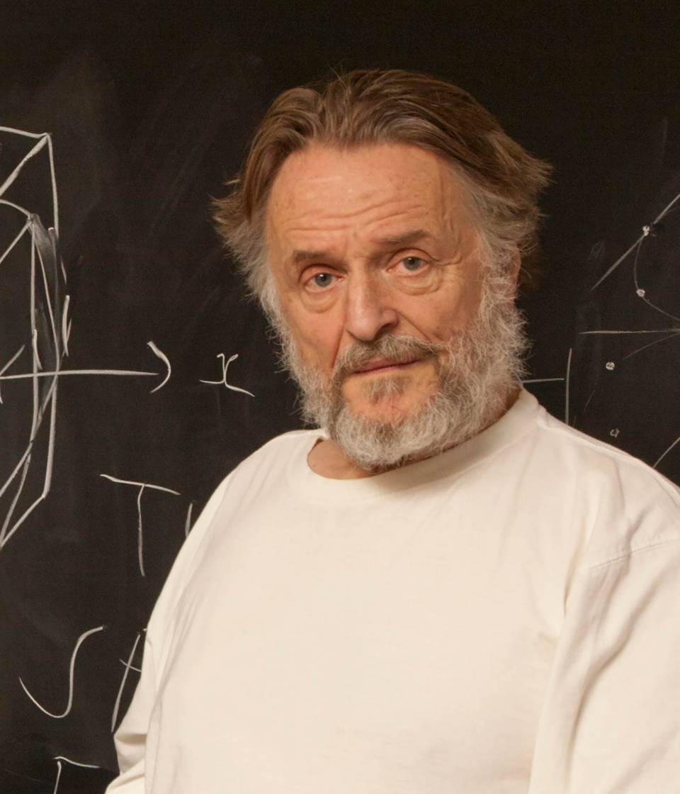
Figure: Left A Glider pattern discovered 1969 by Richard K. Guy. Right. John Horton Conway, creator of Life (1937-2020). The glider is an oscillator that moves diagonally after creation. From the simple rules of Life it’s not obvious that such an object does exist, until you do the necessary computation.

The glider was ‘discovered’ in 1969 by Richard K. Guy. What do we mean by discovered in this context? Well, as soon as the game of life is defined, objects such as the glider do somehow exist, but the many configurations of the game mean that it takes some time for us to see one and know it exists. This means, that despite being the creator, Conway, and despite the rules of the game being simple, and despite the rules being deterministic, we are not ‘omniscient’ in any simplistic sense. It requires computation to ‘discover’ what can exist in this universe once it’s been defined.

Figure: The Gosper glider gun is a configuration that creates gliders. A new glider is released after every 30 turns.

These patterns had to be discovered, in the same way that a scientist might discover a disease, or an explorer a new land. For example, the Gosper glider gun was discovered by Bill Gosper in 1970. It is a pattern that creates a new glider every 30 turns of the game.

Despite widespread interest in Life, some of its patterns were only very recently discovered like the Loafer, discovered in 2013 by Josh Ball. So, despite the game having existed for over forty years, and the rules of the game being simple, there are emergent behaviors that are unknown.

Loafer (2013)

Figure: Left A Loafer pattern discovered by Josh Ball in 2013. Right. John Horton Conway, creator of Life (1937-2020).

Once these patterns are discovered, they are combined (or engineered) to create new Life patterns that do some remarkable things. For example, there’s a life pattern that runs a Turing machine, or more remarkably there’s a Life pattern that runs Life itself.

Figure: The Game of Life running in Life. The video is drawing out recursively showing pixels that are being formed by filling cells with moving spaceships. Each individual pixel in this game of life is made up of \(2048 \times 2048\) pixels called an OTCA metapixel.

To find out more about the Game of Life you can watch this video by Alan Zucconi or read his associated blog post.

Figure: An introduction to the Game of Life by Alan Zucconi.

Contrast this with our situation where in ‘real life’ we don’t know the simple rules of the game, the state space is larger, and emergent behaviors (hurricanes, earthquakes, volcanos, climate change) have direct consequences for our daily lives, and we understand why the process of ‘understanding’ the physical world is so difficult. We also see immediately how much easier we might expect the physical sciences to be than the social sciences, where the emergent behaviors are contingent on highly complex human interactions.

Packing Problems

Figure: Packing 9 squares into a single square. This example is trivially solved. Credit https://erich-friedman.github.io/packing/

Figure: Packing 17 squares into a single square. The optimal solution is sometimes hard to find. Here the side length of the smallest square that holds 17 similarly shaped squares is at least 4.675 times the smaller square. This solution found by John Bidwell in 1997. Credit https://erich-friedman.github.io/packing/

Another example of a problem where the “physics” is understood because it’s really mathematics, is packing problems. Here the mathematics is just geometry, but still we need some form of compute to solve these problems. Erich Friedman’s website contains a host of these problems, only some of which are analytically tractable.

Figure: Packing 10 squares into a single square. This example is proven by Walter Stromquist (Stromquist, 1984). Here \(s=3+\frac{1}{\sqrt{2}}\). Credit https://erich-friedman.github.io/packing/

Bayesian Inference by Rejection Sampling

One view of Bayesian inference is to assume we are given a mechanism for generating samples, where we assume that mechanism is representing an accurate view on the way we believe the world works.

This mechanism is known as our prior belief.

We combine our prior belief with our observations of the real world by discarding all those prior samples that are inconsistent with our observations. The likelihood defines mathematically what we mean by inconsistent with the observations. The higher the noise level in the likelihood, the looser the notion of consistent.

The samples that remain are samples from the posterior.

This approach to Bayesian inference is closely related to two sampling techniques known as rejection sampling and importance sampling. It is realized in practice in an approach known as approximate Bayesian computation (ABC) or likelihood-free inference.

In practice, the algorithm is often too slow to be practical, because most samples will be inconsistent with the observations and as a result the mechanism must be operated many times to obtain a few posterior samples.

However, in the Gaussian process case, when the likelihood also assumes Gaussian noise, we can operate this mechanism mathematically, and obtain the posterior density analytically. This is the benefit of Gaussian processes.

First, we will load in two python functions for computing the covariance function.

Next, we sample from a multivariate normal density (a multivariate Gaussian), using the covariance function as the covariance matrix.

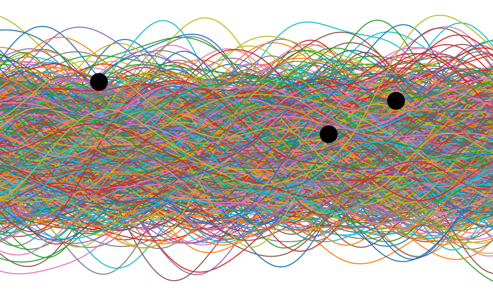
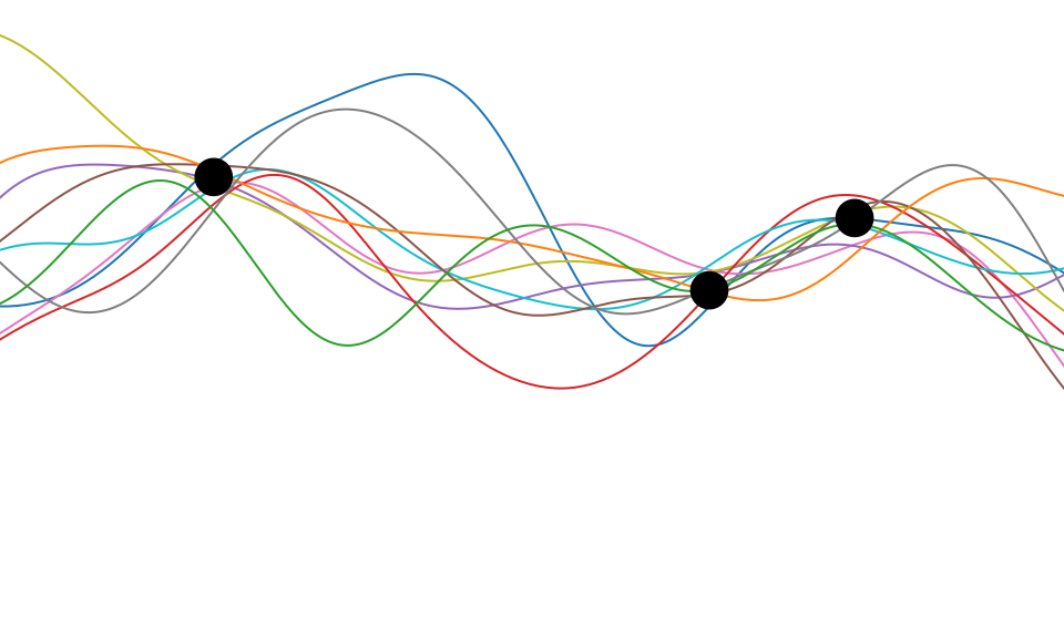
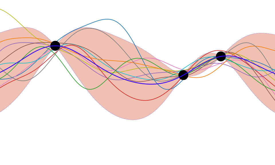
Figure: One view of Bayesian inference is we have a machine for generating samples (the prior), and we discard all samples inconsistent with our data, leaving the samples of interest (the posterior). This is a rejection sampling view of Bayesian inference. The Gaussian process allows us to do this analytically by multiplying the prior by the likelihood.

So, Gaussian processes provide an example of a particular type of model. Or, scientifically, we can think of such a model as a mathematical representation of a hypothesis around data. The rejection sampling view of Bayesian inference can be seen as rejecting portions of that initial hypothesis that are inconsistent with the data. From a Popperian perspective, areas of the prior space are falsified by the data, leaving a posterior space that represents remaining plausible hypotheses.

The flaw with this point of view is that the initial hypothesis space was also restricted. It only contained functions where the instantiated points from the function are jointly Gaussian distributed.

Universe isn’t as Gaussian as it Was

The Planck space craft was a European Space Agency space telescope that mapped the cosmic microwave background (CMB) from 2009 to 2013. The Cosmic Microwave Background is the first observable echo we have of the big bang. It dates to approximately 400,000 years after the big bang, at the time the Universe was approximately \(10^8\) times smaller and the temperature of the Universe was high, around \(3 \times 10^8\) degrees Kelvin. The Universe was in the form of a hydrogen plasma. The echo we observe is the moment when the Universe was cool enough for protons and electrons to combine to form hydrogen atoms. At this moment, the Universe became transparent for the first time, and photons could travel through space.

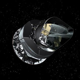
Figure: Artist’s impression of the Planck spacecraft which measured the Cosmic Microwave Background between 2009 and 2013.

The objective of the Planck spacecraft was to measure the anisotropy and statistics of the Cosmic Microwave Background. This was important, because if the standard model of the Universe is correct the variations around the very high temperature of the Universe of the CMB should be distributed according to a Gaussian process.¹ Currently our best estimates show this to be the case (Elsner et al., 2016, 2015; Jaffe et al., 1998; Pontzen and Peiris, 2010).

To the high degree of precision that we could measure with the Planck space telescope, the CMB appears to be a Gaussian process. The parameters of its covariance function are given by the fundamental parameters of the Universe, for example the amount of dark matter and matter in the Universe.

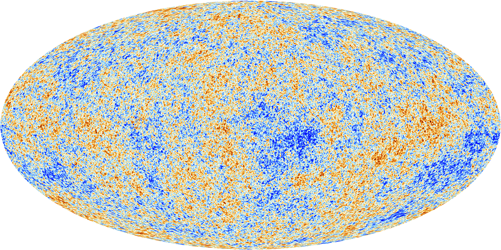
Figure: The cosmic microwave background is, to a very high degree of precision, a Gaussian process. The parameters of its covariance function are given by fundamental parameters of the universe, such as the amount of dark matter and mass.

Simulating a CMB Map

The simulation was created by Boris Leistedt, see the original Jupyter notebook here.

Here we use that code to simulate our own universe and sample from what it looks like.

First, we install some specialist software as well as matplotlib, scipy, numpy we require

• camb: http://camb.readthedocs.io/en/latest/
• healpy: https://healpy.readthedocs.io/en/latest/

%pip install camb

%pip install healpy

import healpy as hp

import camb
from camb import model, initialpower

Now we use the theoretical power spectrum to design the covariance function.

nside = 512  # Healpix parameter, giving 12*nside**2 equal-area pixels on the sphere.
lmax = 3*nside # band-limit. Should be 2*nside < lmax < 4*nside to get information content.

Now we design our Universe. It is parameterized according to the \(\Lambda\)CDM model. The variables are as follows. H0 is the Hubble parameter (in Km/s/Mpc). The ombh2 is Physical Baryon density parameter. The omch2 is the physical dark matter density parameter. mnu is the sum of the neutrino masses (in electron Volts). omk is the \(\Omega_k\) is the curvature parameter, which is here set to 0, giving the minimal six parameter Lambda-CDM model. tau is the reionization optical depth.

Then we set ns, the “scalar spectral index”. This was estimated by Planck to be 0.96. Then there’s r, the ratio of the tensor power spectrum to scalar power spectrum. This has been estimated by Planck to be under 0.11. Here we set it to zero. These parameters are associated with inflation.

# Mostly following http://camb.readthedocs.io/en/latest/CAMBdemo.html with parameters from https://en.wikipedia.org/wiki/Lambda-CDM_model

pars = camb.CAMBparams()
pars.set_cosmology(H0=67.74, ombh2=0.0223, omch2=0.1188, mnu=0.06, omk=0, tau=0.066)
pars.InitPower.set_params(ns=0.96, r=0)

Having set the parameters, we now use the python software “Code for Anisotropies in the Microwave Background” to get the results.

pars.set_for_lmax(lmax, lens_potential_accuracy=0);
results = camb.get_results(pars)
powers = results.get_cmb_power_spectra(pars)
totCL = powers['total']
unlensedCL = powers['unlensed_scalar']

ells = np.arange(totCL.shape[0])
Dells = totCL[:, 0]
Cells = Dells * 2*np.pi / ells / (ells + 1)  # change of convention to get C_ell
Cells[0:2] = 0

cmbmap = hp.synfast(Cells, nside, 
                 lmax=lmax, mmax=None, alm=False, pol=False, 
                 pixwin=False, fwhm=0.0, sigma=None, new=False, verbose=True)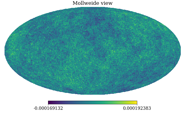

Figure: A simulation of the Cosmic Microwave Background obtained through sampling from the relevant Gaussian process covariance (in polar co-ordinates).

The world we see today, of course, is not a Gaussian process. There are many discontinuities, for example, in the density of matter, and therefore in the temperature of the Universe.

\(=f\Bigg(\)\(\Bigg)\)

Figure: What we observe today is some non-linear function of the cosmic microwave background.

We can think of today’s observed Universe, though, as a being a consequence of those temperature fluctuations in the CMB. Those fluctuations are only order \(10^{-6}\) of the scale of the overall temperature of the Universe. But minor fluctuations in that density are what triggered the pattern of formation of the Galaxies. They determined how stars formed and created the elements that are the building blocks of our Earth (Vogelsberger et al., 2020).

Those cosmological simulations are based on a relatively simple set of ‘rules’ that stem from our understanding of natural laws. These ‘rules’ are mathematical abstractions of the physical world. Representations of behavior in mathematical form that capture the interaction forces between particles. The grand aim of physics has been to unify these rules into a single unifying theory. Popular understanding of this quest developed because of Stephen Hawking’s book, “A Brief History of Time”. The idea of these laws as ‘ultimate causes’ has given them a pseudo religious feel, see for example Paul Davies’s book “The Mind of God” which comes from a quotation form Stephen Hawking.

If we do discover a theory of everything … it would be the ultimate triumph of human reason-for then we would truly know the mind of God

Stephen Hawking in A Brief History of Time 1988

This is an entrancing quote, that seems to work well for selling books (A Brief History of Time sold over 10 million copies), but as Laplace has already pointed out to us, the Universe doesn’t work quite so simply as that. Commonly, God is thought to be omniscient, but having a grand unifying theory alone doesn’t give us omniscience.

Laplace’s demon still applies. Even if we had a grand unifying theory, which encoded “all the forces that set nature in motion” we have an amount of work left to do in any quest for ‘omniscience’.

We may regard the present state of the universe as the effect of its past and the cause of its future. An intellect which at a certain moment would know all forces that set nature in motion, and all positions of all items of which nature is composed, …

… if this intellect were also vast enough to submit these data to analysis, it would embrace in a single formula the movements of the greatest bodies of the universe and those of the tiniest atom; for such an intellect nothing would be uncertain and the future just like the past would be present before its eyes.

— Pierre Simon Laplace (Laplace, 1814)

We summarized this notion as \[ \text{data} + \text{model} \stackrel{\text{compute}}{\rightarrow} \text{prediction} \] As we pointed out, there is an irony in Laplace’s demon forming the cornerstone of a movement known as ‘determinism’, because Laplace wrote about this idea in an essay on probabilities. The more important quote in the essay was

Laplace’s Gremlin

The curve described by a simple molecule of air or vapor is regulated in a manner just as certain as the planetary orbits; the only difference between them is that which comes from our ignorance. Probability is relative, in part to this ignorance, in part to our knowledge. We know that of three or greater number of events a single one ought to occur; but nothing induces us to believe that one of them will occur rather than the others. In this state of indecision it is impossible for us to announce their occurrence with certainty. It is, however, probable that one of these events, chosen at will, will not occur because we see several cases equally possible which exclude its occurrence, while only a single one favors it.

— Pierre-Simon Laplace (Laplace, 1814), pg 5

The representation of ignorance through probability is the true message of Laplace, I refer to this message as “Laplace’s gremlin”, because it is the gremlin of uncertainty that interferes with the demon of determinism to mean that our predictions are not deterministic.

Our separation of the uncertainty into the data, the model and the computation give us three domains in which our doubts can creep into our ability to predict. Over the last three lectures we’ve introduced some of the basic tools we can use to unpick this uncertainty. You’ve been introduced to, (or have yow reviewed) Bayes’ rule. The rule, which is a simple consequence of the product rule of probability, is the foundation of how we update our beliefs in the presence of new information.

The real point of Laplace’s essay was that we don’t have access to all the data, we don’t have access to a complete physical understanding, and as the example of the Game of Life shows, even if we did have access to both (as we do for “Conway’s universe”) we still don’t have access to all the compute that we need to make deterministic predictions. There is uncertainty in the system which means we can’t make precise predictions.

Gremlins are imaginary creatures used as an explanation of failure in aircraft, causing crashes. In that sense the Gremlin represents the uncertainty that a pilot felt about what might go wrong in a plane which might be “theoretically sound” but in practice is poorly maintained or exposed to conditions that take it beyond its design criteria. Laplace’s gremlin is all the things that your model, data and ability to compute don’t account for bringing about failures in your ability to predict. Laplace’s gremlin is the uncertainty in the system.

Figure: Gremlins are seen as the cause of a number of challenges in this World War II poster.

Carl Henrik described how a prior probability \(p(\boldsymbol{ \theta})\) represents our hypothesis about the way the world might behave. This can be combined with a likelihood through the process of multiplication. Correctly normalized, this gives an updated hypothesis that represents our posterior belief about the model in the light of the data.

There is a nice symmetry between this approach and how Karl Popper describes the process of scientific discovery. In Conjectures and Refutations (Popper (1963)), Popper describes the process of scientific discovery as involving hypothesis and experiment. In our description hypothesis maps onto the model. The model is an abstraction of the hypothesis, represented for example as a set of mathematical equations, a computational description, or an analogous system (physical system). The data is the product of previous experiments, our readings, our observation of the world around us. We can combine these to make a prediction about what we might expect the future to hold. Popper’s view on the philosophy of science was that the prediction should be falsifiable.

We can see this process as a spiral driving forward, importantly Popper relates the relationship between hypothesis (model) and experiment (predictions) as akin to the relationship between the chicken and the egg. Which comes first? The answer is that they co-evolve together.

Figure: Experiment, analyze and design is a flywheel of knowledge that is the dual of the model, data and compute. By running through this spiral, we refine our hypothesis/model and develop new experiments which can be analyzed to further refine our hypothesis.

Figure: The sets of different models. There are all the models in the Universe we might like to work with. Then there are those models that are computable e.g., by a Turing machine. Then there are those which are analytical tractable. I.e., where the solution might be found analytically. Finally, there are Gaussian processes, where the joint distribution of the states in the model is Gaussian.

The approach we’ve taken to the model so far has been severely limiting. By constraining ourselves to models for which the mathematics of probability is tractable, we severely limit what we can say about the universe.

Although Bayes’ rule only implies multiplication of probabilities, to acquire the posterior we also need to normalize. Very often it is this normalization step that gets in the way. The normalization step involves integration over the updated hypothesis space, to ensure the updated posterior prediction is correct.

We can map the process of Bayesian inference onto the \(\text{model} + \text{data}\) perspective in the following way. We can see the model as the prior, the data as the likelihood and the prediction as the posterior².

So, if we think of our model as incorporating what we know about the physical problem of interest (from Newton, or Bernoulli or Laplace or Einstein or whoever) and the data as being the observations (e.g., from Piazzi’s telescope or a particle accelerator) then we can make predictions about what we might expect to happen in the future by combining the two. It is those predictions that Popper sees as important in verifying the scientific theory (which is incorporated in the model).

But while Gaussian processes are highly flexible non-parametric function models, they are not going to be sufficient to capture the type of physical processes we might expect to encounter in the real world. To give a sense, let’s consider a few examples of the phenomena we might want to capture, either in the scientific world, or in real world decision making.

Precise Physical Laws

We’ve already reviewed the importance of Newton’s laws in forging our view of science: we mentioned the influence Christiaan Huygens’ work on collisions had on Daniel Bernoulli in forming the kinetic theory of gases. These ideas inform many of the physical models we have today around a number of natural phenomena. The MET Office supercomputer in Exeter spends its mornings computing the weather across the world its afternoons modelling climate scenarios. It uses the same set of principles that Newton described, and Bernoulli explored for gases. They are encoded in the Navier-Stokes equations. Differential equations that govern the flow of compressible and incompressible fluids. As well as predicting our weather, these equations are used in fluid dynamics models to understand the flight of aircraft, the driving characteristics of racing cars and the efficiency of gas turbine engines.

This broad class of physical models, or ‘natural laws’ is probably the closest to what Laplace was referring to in the demon. The search for unifying physical laws that dictate everything we observe around us has gone on. Alongside Newton we must mention James Clerk Maxwell, who unified electricity and magnetism in one set of equations that were inspired by the work and ideas of Michael Faraday. And still today we look for unifying equations that bring together in a single mathematical model the ‘natural laws’ we observe. One equation that for Laplace would be “all forces that set nature in motion”. We can think of this as our first time of physical model, a ‘precise model’ of the known laws of our Universe, a model where we expect that the mapping from the mathematical abstraction to the physical reality is ‘exact’.³

Abstraction and Emergent Properties

Figure: A scale of different simulations we might be interested in when modelling the physical world. The scale is \(\log_{10}\) meters. The scale reflects something about the level of granularity where we might choose to know “all positions of all items of which nature is composed”.

Unfortunately, even if such an equation were to exist, we would be unlikely to know “all positions of all items of which nature is composed”. A good example here is computational systems biology. In that domain we are interested in understanding the underlying function of the cell. These systems sit somewhere between the two extremes that Laplace described: “the movements of the greatest bodies of the universe and those of the smallest atom”.

When the smallest atom is considered, we need to introduce uncertainty. We again turn to a different work of Maxwell, building on Bernoulli’s kinetic theory of gases we end up with probabilities for representing the location of the ‘molecules of air’. Instead of a deterministic location for these particles we represent our belief about their location in a distribution.

Computational systems biology is a world of micro-machines, built of three dimensional foldings of strings of proteins. There are spindles (stators) and rotors (e.g. ATP Synthase), there are small copying machines (e.g. RNA Polymerase) there are sequence to sequence translators (Ribosomes). The cells store information in DNA but have an ecosystem of structures and messages being built and sent in proteins and RNA. Unpicking these structures has been a major preoccupation of biology. That is knowing where the atoms of these molecules are in the structure, and how the parts of the structure move when these small micro-machines are carrying out their roles.

We understand most (if not all) of the physical laws that drive the movements of these molecules, but we don’t understand all the actions of the cell, nor can we intervene reliably to improve things. So, even in the case where we have a good understanding of the physical laws, Laplace’s gremlin emerges in our knowledge of “the positions of all items of which nature is composed”.

Molecular Dynamics Simulations

By understanding and simulating the physics, we can recreate operations that are happening at the level of proteins in the human cell. V-ATPase is an enzyme that pumps protons. But at the microscopic level it’s a small machine. It produces ATP in response to a proton gradient. A paper in Science Advances (Roh et al., 2020) simulates the functioning of these proteins that operate across the cell membrane. This makes these proteins difficult to crystallize, the response to this challenge is to use a simulation which (somewhat) abstracts the processes. You can also check this blog post from the paper’s press release.

Figure: The V-ATPase enzyme pumps proteins across membranes. This molecular dynamics simulation was published in Science Advances (Roh et al., 2020). The scale is roughly \(10^{-8} m\).

Quantum Mechanics

Alternatively, we can drop down a few scales and consider simulation of the Schrödinger equation. Intractabilities in the many-electron Schrödinger equation have been addressed using deep neural networks to speed up the solution enabling simulation of chemical bonds (Pfau et al., 2020). The PR-blog post is also available. The paper uses a neural network to model the quantum state of a number of electrons.

Figure: The many-electron Schrödinger equation is important in understanding how Chemical bonds are formed.

Each of these simulations have the same property of being based on a set of (physical) rules about how particles interact. But one of the interesting characteristics of such systems is how the properties of the system are emergent as the dynamics are allowed to continue.

These properties cannot be predicted without running the physics, or the equivalently the equation. Computation is required. And often the amount of computation that is required is prohibitive.

Accelerate Programme

The Computer Lab is hosting a new initiative, funded by Schmidt Futures, known as the Accelerate Programme for Scientific Discovery. The aim is to address scientific challenges, and accelerate the progress of research, through using tools in machine learning.

We now have four fellows appointed, each of whom works at the interface of machine learning and scientific discovery. They are using the ideas around machine learning modelling to drive their scientific research.

For example, Bingqing Cheng, one of the Department’s former DECAF Fellows has used neural network accelerated molecular dynamics simulations to understand a new form of metallic hydrogen, likely to occur at the heart of stars (Cheng et al., 2020). The University’s press release is here.

On her website Bingqing quotes Paul Dirac.

The fundamental laws necessary for the mathematical treatment of a large part of physics and the whole of chemistry are thus completely known, and the difficulty lies only in the fact that application of these laws leads to equations that are too complex to be solved.

..approximate practical methods of applying quantum mechanics should be developed, which can lead to an explanation of the main features of complex atomic systems without too much computation.

— Paul Dirac (6 April 1929)

Bingqing has now taken a position at IST Austria.

Our four current Accelerate fellows are Challenger Mishra, a physicist interested in string theory and quantizing gravity. Sarah Morgan from the Brain Mapping Unit, who is focused on predicting psychosis trajectories, Soumya Bannerjee who focuses on complex systems and healthcare and Sam Nallaperuma who the interface of machine learning and biology with particular interests in emergent behavior in complex systems.

For those interested in Part III/MPhil projects, you can see their project suggestions on this page.

Related Approaches

While this module is mainly focusing on emulation as a route to bringing machine learning closer to the physical world, I don’t want to give the impression that’s the only approach. It’s worth bearing in mind three important domains of machine learning (and statistics) that we also could have explored.

• Probabilistic Programming
• Approximate Bayesian Computation
• Causal inference

Each of these domains also brings a lot to the table in terms of understanding the physical world.

Probabilistic Programming

Probabilistic programming is an idea that, from our perspective, can be summarized as follows. What if, when constructing your simulator, or your model, you used a programming language that was aware of the state variables and the probability distributions. What if this language could ‘compile’ the program into code that would automatically compute the Bayesian posterior for you?

This is the objective of probabilistic programming. The idea is that you write your model in a language, and that language is automatically converted into the different modelling codes you need to perform Bayesian inference.

The ideas for probabilistic programming originate in BUGS. The software was developed at the MRC Biostatistics Unit here in Cambridge in the early 1990s, by among others, Sir David Spiegelhalter. Carl Henrik covered in last week’s lecture some of the approaches for approximate inference. BUGS uses Gibbs sampling. Gibbs sampling, however, can be slow to converge when there are strong correlations in the posterior between variables.

The descendent of BUGS that is probably most similar in the spirit of its design is Stan. Stan came from researchers at Columbia University and makes use of a variant of Hamiltonian Monte Carlo called the No-U-Turn sampler. It builds on automatic differentiation for the gradients it needs. It’s all written in C++ for speed, but has interfaces to Python, R, Julia, MATLAB etc. Stan has been highly successful during the Coronavirus pandemic, with a number of epidemiological simulations written in the language, for example see this blog post.

Other probabilistic programming languages of interest include those that make use of variational approaches (such as pyro) and allow use of neural network components.

One important probabilistic programming language being developed is Turing, one of the key developers is Hong Ge who is a Senior Research Associate in Cambridge Engineering.

Approximate Bayesian Computation

We reintroduced Gaussian processes at the start of this lecture by sampling from the Gaussian process and matching the samples to data, discarding those that were distant from our observations. This approach to Bayesian inference is the starting point for approximate Bayesian computation or ABC.

The idea is straightforward, if we can measure ‘closeness’ in some relevant fashion, then we can sample from our simulation, compare our samples to real world data through ‘closeness measure’ and eliminate samples that are distant from our data. Through appropriate choice of closeness measure, our samples can be viewed as coming from an approximate posterior.

My Sheffield colleague, Rich Wilkinson, was one of the pioneers of this approach during his PhD in the Statslab here in Cambridge. You can hear Rich talking about ABC at NeurIPS in 2013 here.

Figure: Rich Wilkinson giving a Tutorial on ABC at NeurIPS in 2013. Unfortunately, they’ve not synchronised the slides with the tutorial. You can find the slides separately here.

Causality

Figure: Judea Pearl and Elias Bareinboim giving a Tutorial on Causality at NeurIPS in 2013. Again, the slides aren’t synchronised, but you can find them separately here.

All these approaches offer a lot of promise for developing machine learning at the interface with science but covering each in detail would require four separate modules. We’ve chosen to focus on the emulation approach, for two principal reasons. Firstly, it’s conceptual simplicity. Our aim is to replace all or part of our simulation with a machine learning model. Typically, we’re going to want uncertainties as part of that representation. That explains our focus on Gaussian process models. Secondly, the emulator method is flexible. Probabilistic programming requires that the simulator has been built in a particular way, otherwise we can’t compile the program. Finally, the emulation approach can be combined with any of the existing simulation approaches. For example, we might want to write our emulators as probabilistic programs. Or we might do causal analysis on our emulators, or we could speed up the simulation in ABC through emulation.

Conclusion

We’ve introduced the notion of a simulator. A body of computer code that expresses our understanding of a particular physical system. We introduced such simulators through physical laws, such as laws of gravitation or electro-magnetism. But we soon saw that in many simulations those laws become abstracted, and the simulation becomes more phenomological.

Even full knowledge of all laws does not give us access to ‘the mind of God’, because we are lacking information about the data, and we are missing the compute. These challenges further motivate the need for abstraction, and we’ve seen examples of where such abstractions are used in practice.

The example of Conway’s Game of Life highlights how complex emergent phenomena can require significant computation to explore.

Thanks!

For more information on these subjects and more you might want to check the following resources.

• twitter: @lawrennd
• podcast: The Talking Machines
• newspaper: Guardian Profile Page
• blog: http://inverseprobability.com

References