Deep Architectures

ML Foundations Course Notebook Setup

Neural Networks

Shallow and Deep Learning

From Basis Functions to Neural Networks (JAX)

Parametric Basis Functions

Multi-Layer Perceptron as Stacked Bases

Loss and Training (JAX grad/jit)

Demo: Olympics Data with a Neural Network

Discussion

Deep Neural Network

Deep Neural Network

Mathematically

\[ \begin{align*} \mathbf{ h}_{1} &= \phi\left(\mathbf{W}_1 \mathbf{ x}\right)\\ \mathbf{ h}_{2} &= \phi\left(\mathbf{W}_2\mathbf{ h}_{1}\right)\\ \mathbf{ h}_{3} &= \phi\left(\mathbf{W}_3 \mathbf{ h}_{2}\right)\\ f&= \mathbf{ w}_4 ^\top\mathbf{ h}_{3} \end{align*} \]

Neural Network Prediction Function

Overparameterised Systems

• Neural networks are highly overparameterised.
• If we could examine their Hessian at “optimum”
  • Very low (or negative) eigenvalues.
  • Error function is not sensitive to changes in parameters.
  • Implies parmeters are badly determined

Whence Generalisation?

• Not enough regularisation in our objective functions to explain.
• Neural network models are not using traditional generalisation approaches.
• The ability of these models to generalise must be coming somehow from the algorithm*
• How to explain it and control it is perhaps the most interesting theoretical question for neural networks.

Generalization and Overfitting

• How does the model perform on previously unseen data?

Validation and Model Selection

• Selecting model at the validation step

Difficult Trap

• Vital that you avoid test data in training.
• Validation data is different from test data.

Olympic Marathon Data

Gold medal times for Olympic Marathon since 1896. Marathons before 1924 didn’t have a standardized distance. Present results using pace per km. In 1904 Marathon was badly organized leading to very slow times.

Image from Wikimedia Commons

Olympic Marathon Data

Hold Out Validation on Olympic Marathon Data

Overfitting

• Increase number of basis functions we obtain a better ‘fit’ to the data.
• How will the model perform on previously unseen data?
• Let’s consider predicting the future.

Future Prediction: Extrapolation

❮ ❯

Extrapolation

• Here we are training beyond where the model has learnt.
• This is known as extrapolation.
• Extrapolation is predicting into the future here, but could be:
  • Predicting back to the unseen past (pre 1892)
  • Spatial prediction (e.g. Cholera rates outside Manchester given rates inside Manchester).

Interpolation

• Predicting the wining time for 1946 Olympics is interpolation.
• This is because we have times from 1936 and 1948.
• If we want a model for interpolation how can we test it?
• One trick is to sample the validation set from throughout the data set.

Future Prediction: Interpolation

❮ ❯

Choice of Validation Set

• The choice of validation set should reflect how you will use the model in practice.
• For extrapolation into the future we tried validating with data from the future.
• For interpolation we chose validation set from data.
• For different validation sets we could get different results.

Bias Variance Decomposition

Generalisation error \[\begin{align*} R(\mathbf{ w}) = & \int \left(y- f^*(\mathbf{ x})\right)^2 \mathbb{P}(y, \mathbf{ x}) \text{d}y\text{d}\mathbf{ x}\\ & \triangleq \mathbb{E}\left[ \left(y- f^*(\mathbf{ x})\right)^2 \right]. \end{align*}\]

Decompose

Decompose as \[ \begin{align*} \mathbb{E}\left[ \left(y- f(\mathbf{ x})\right)^2 \right] = & \text{bias}\left[f^*(\mathbf{ x})\right]^2 \\ & + \text{variance}\left[f^*(\mathbf{ x})\right] \\ \\ &+\sigma^2, \end{align*} \]

Bias

• Given by \[ \text{bias}\left[f^*(\mathbf{ x})\right] = \mathbb{E}\left[f^*(\mathbf{ x})\right] - f(\mathbf{ x}) \]

• Error due to bias comes from a model that’s too simple.

Variance

• Given by \[ \text{variance}\left[f^*(\mathbf{ x})\right] = \mathbb{E}\left[\left(f^*(\mathbf{ x}) - \mathbb{E}\left[f^*(\mathbf{ x})\right]\right)^2\right]. \]

• Slight variations in the training set cause changes in the prediction. Error due to variance is error in the model due to an overly complex model.

Overfitting

Alex Ihler on Polynomials and Overfitting

From Shallow to Deep

\[ f(\mathbf{ x}; \mathbf{W}) = \mathbf{ w}_4 ^\top\phi\left(\mathbf{W}_3 \phi\left(\mathbf{W}_2\phi\left(\mathbf{W}_1 \mathbf{ x}\right)\right)\right). \]

Gradient-based optimization

\[ \mathscr{L}(\theta) = \sum_{n=1}^N \ell(y_n, f(x_n, \theta)) \]

\[ \theta_{t+1} = \theta_t - \eta \nabla_\theta \mathcal{L}(\theta) \]

Basic Multilayer Perceptron

\[ \small f_L(x) = \boldsymbol{ \phi}\left(b_L + W_L \boldsymbol{ \phi}\left(b_{L-1} + W_{L-1} \boldsymbol{ \phi}\left( \cdots \boldsymbol{ \phi}\left(b_1 + W_1 x\right) \cdots \right)\right)\right) \]

Recursive MLP Definition

\[\begin{align} f_l(x) &= \boldsymbol{ \phi}\big(W_l f_{l-1}(x) + b_l\big),\quad l=1,\dots,L\\ f_0(x) &= x \end{align}\]

Rectified Linear Unit

Shallow ReLU Networks

\[\begin{align} \mathbf{h}(x) &= \operatorname{ReLU}(\mathbf{w}_1 x - \mathbf{b}_1)\\ f(x) &= \mathbf{w}_2^{\top} \, \mathbf{h}(x) \end{align}\]

Complexity (1D): number of kinks \(\propto\) width of network.

Depth vs Width: Representation Power

• Single hidden layer: number of kinks \(\approx O(\text{width})\)
• Deep ReLU networks: kinks \(\approx O(2^{\text{depth}})\)

Sawtooth Construction

\[\begin{align} f_l(x) &= 2\vert f_{l-1}(x)\vert - 2, \quad f_0(x) = x\\ f_l(x) &= 2 \operatorname{ReLU}(f_{l-1}(x)) + 2 \operatorname{ReLU}(-f_{l-1}(x)) - 2 \end{align}\]

Complexity (1D): number of kinks \(\approx O(2^{\text{depth}})\).

Higher-dimensional Geometry

• Regions: piecewise-linear, often triangular/polygonal in 2D
• Continuity arises despite stitching flat regions
• Early layers: few regions; later layers: many more

Generalisation in Deep Networks

• Classical view: model class + loss determine generalisation
• Deep view: optimisation algorithm (SGD variants) also determines which interpolating solution is found
• Phenomena: double descent; NTK/infinite-width limits; role of initialisation and gradient noise

Factors Affecting Generalisation

• Data representativeness: train/test distribution alignment
• Number of training points: more samples narrow feasible solutions
• Model class size: larger classes require more data

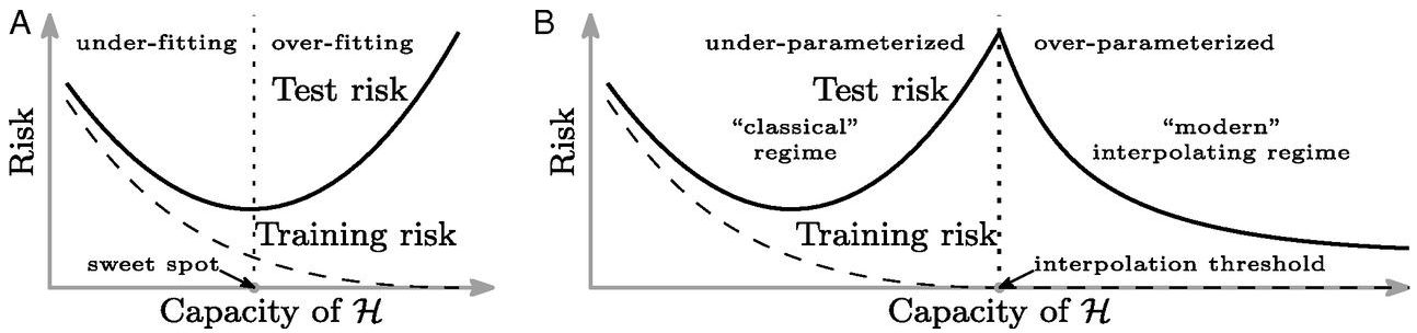
Double Descent

Neural Tangent Kernel

• Consider very wide neural networks.
• Consider particular initialisation.
• Deep neural network is regularising with a particular kernel.
• This is known as the neural tangent kernel (Jacot et al., 2018).

Regularization in Optimization

• Gradient flow methods allow us to study nature of optima.
• In particular systems, with given initialisations, we can show L1 and L2 norms are minimised.
• In other cases the rank of \(\mathbf{W}\) is minimised.
• Questions remain over the nature of this regularisation in neural networks.

Deep Linear Models

\[ f(\mathbf{ x}; \mathbf{W}) = \mathbf{W}_4 \mathbf{W}_3 \mathbf{W}_2 \mathbf{W}_1 \mathbf{ x}. \]

\[ \mathbf{W}= \mathbf{W}_4 \mathbf{W}_3 \mathbf{W}_2 \mathbf{W}_1 \]

Chain Rule and Back Propgation

Matrix Vector Chain Rule

Matrix Stacking

Kronecker Products

{In most cases Kronecker products they arise below they are later removed using this relationship \[ (\mathbf{E}:)^{\top} \mathbf{F} \otimes \mathbf{G}=\left(\left(\mathbf{G}^{\top} \mathbf{E F}\right):\right)^{\top} \] this form typically arises whenever the chain rule is applied, \[ \frac{\text{d} E}{\text{d} \mathbf{H}:} \frac{\text{d} \mathbf{H}:}{\text{d} \mathbf{J}:}=\frac{\text{d} E}{\text{d} \mathbf{J}:}, \]

as we normally find that \(\frac{\text{d} \mathbf{H}}{\text{d} \mathbf{J}}\) has the form of a Kronecker product, \(\frac{\text{d} \mathbf{H}}{\text{d} \mathbf{J}}=\mathbf{F} \otimes \mathbf{G}\) and we expect the result of \(\frac{\text{d} E}{\text{d} \mathbf{H}}\) and \(\frac{\text{d} E}{\text{d} \mathbf{J}}\) to be in the form \((\mathbf{E}:)^{\mathbf{T}}\). The following two identities for Kronecker products will also prove useful. \[ \mathbf{F}^{\top} \otimes \mathbf{G}^{\top}=(\mathbf{F} \otimes \mathbf{G})^{\top} \] and \[ (\mathbf{E} \otimes \mathbf{G})(\mathbf{F} \otimes \mathbf{H})=\mathbf{E F} \otimes \mathbf{G H} \] Generally we will use two ways of writing the derivative of a scalar with respect to a matrix, \(\frac{\text{d} E}{\text{d} \mathbf{J}}\) and \(\frac{\text{d} E}{\text{d} \mathbf{J}}\), the first being a row vector and the second is a matrix of the same dimension of \(\mathbf{J}\). The second representation is more convenient for summarising the result, the first is easier to wield when computing the result. The equivalence of the representations is given by \[ \frac{\text{d} E}{\text{d} \mathbf{J}:}=\left(\left(\frac{\text{d} E}{\text{d} \mathbf{J}}\right):\right)^{\top}. \]

Any other results used for matrix differentiation and not explicitly given here may be found in Brookes [2005].

Useful Multivariate Derivatives

Chain Rule for Neural Networks

Evaluating Derivatives

\[ \frac{\text{d} \mathbf{ f}_L}{\text{d} \mathbf{ w}} = \frac{\text{d} \mathbf{ f}_L}{\text{d} \mathbf{ f}_{L-1}} \frac{\text{d} \mathbf{ f}_{L-1}}{\text{d} \mathbf{ f}_{L-2}} \frac{\text{d} \mathbf{ f}_{L-2}}{\text{d} \mathbf{ f}_{L-3}} \cdots \frac{\text{d} \mathbf{ f}_3}{\text{d} \mathbf{ f}_{2}} \frac{\text{d} \mathbf{ f}_2}{\text{d} \mathbf{ f}_{1}} \frac{\text{d} \mathbf{ f}_1}{\text{d} \mathbf{ w}} \]

\[ \small \frac{\text{d} \mathbf{ f}_L}{\text{d} \mathbf{ w}} = \frac{\text{d} \mathbf{ f}_L}{\text{d} \mathbf{ f}_{L-1}} \left( \frac{\text{d} \mathbf{ f}_{L-1}}{\text{d} \mathbf{ f}_{L-2}} \left( \frac{\text{d} \mathbf{ f}_{L-2}}{\text{d} \mathbf{ f}_{L-3}} \cdots \left( \frac{\text{d} \mathbf{ f}_3}{\text{d} \mathbf{ f}_{2}} \left( \frac{\text{d} \mathbf{ f}_2}{\text{d} \mathbf{ f}_{1}} \frac{\text{d} \mathbf{ f}_1}{\text{d} \mathbf{ w}} \right) \right) \cdots \right) \right) \]

Or like this?

\[ \frac{\text{d} \mathbf{ f}_L}{\text{d} \mathbf{ w}} = \frac{\text{d} \mathbf{ f}_L}{\text{d} \mathbf{ f}_{L-1}} \frac{\text{d} \mathbf{ f}_{L-1}}{\text{d} \mathbf{ f}_{L-2}} \frac{\text{d} \mathbf{ f}_{L-2}}{\text{d} \mathbf{ f}_{L-3}} \cdots \frac{\text{d} \mathbf{ f}_3}{\text{d} \mathbf{ f}_{2}} \frac{\text{d} \mathbf{ f}_2}{\text{d} \mathbf{ f}_{1}} \frac{\text{d} \mathbf{ f}_1}{\text{d} \mathbf{ w}} \]

\[ \small \frac{\text{d} \mathbf{ f}_L}{\text{d} \mathbf{ w}} = \left( \left( \cdots \left( \left( \frac{\text{d} \mathbf{ f}_L}{\text{d} \mathbf{ f}_{L-1}} \frac{\text{d} \mathbf{ f}_{L-1}}{\text{d} \mathbf{ f}_{L-2}} \right) \frac{\text{d} \mathbf{ f}_{L-2}}{\text{d} \mathbf{ f}_{L-3}} \right) \cdots \frac{\text{d} \mathbf{ f}_3}{\text{d} \mathbf{ f}_{2}} \right) \frac{\text{d} \mathbf{ f}_2}{\text{d} \mathbf{ f}_{1}} \right) \frac{\text{d} \mathbf{ f}_1}{\text{d} \mathbf{ w}} \]

Or in a funky way?

\[ \frac{\text{d} \mathbf{ f}_L}{\text{d} \mathbf{ w}} = \frac{\text{d} \mathbf{ f}_L}{\text{d} \mathbf{ f}_{L-1}} \frac{\text{d} \mathbf{ f}_{L-1}}{\text{d} \mathbf{ f}_{L-2}} \frac{\text{d} \mathbf{ f}_{L-2}}{\text{d} \mathbf{ f}_{L-3}} \cdots \frac{\text{d} \mathbf{ f}_3}{\text{d} \mathbf{ f}_{2}} \frac{\text{d} \mathbf{ f}_2}{\text{d} \mathbf{ f}_{1}} \frac{\text{d} \mathbf{ f}_1}{\text{d} \mathbf{ w}} \]

\[ \small \frac{\text{d} \mathbf{ f}_L}{\text{d} \mathbf{ w}} = \frac{\text{d} \mathbf{ f}_L}{\text{d} \mathbf{ f}_{L-1}} \left( \left( \left( \frac{\text{d} \mathbf{ f}_{L-1}}{\text{d} \mathbf{ f}_{L-2}} \right) \frac{\text{d} \mathbf{ f}_{L-2}}{\text{d} \mathbf{ f}_{L-3}} \right) \left( \left( \cdots \frac{\text{d} \mathbf{ f}_3}{\text{d} \mathbf{ f}_{2}} \right) \frac{\text{d} \mathbf{ f}_2}{\text{d} \mathbf{ f}_{1}} \right) \right)\frac{\text{d} \mathbf{ f}_1}{\text{d} \mathbf{ w}} \]

Automatic differentiation

Forward-mode

\[ \small \frac{\text{d} \mathbf{ f}_L}{\text{d} \mathbf{ w}} = \frac{\text{d} \mathbf{ f}_L}{\text{d} \mathbf{ f}_{L-1}} \left( \frac{\text{d} \mathbf{ f}_{L-1}}{\text{d} \mathbf{ f}_{L-2}} \left( \frac{\text{d} \mathbf{ f}_{L-2}}{\text{d} \mathbf{ f}_{L-3}} \cdots \left( \frac{\text{d} \mathbf{ f}_3}{\text{d} \mathbf{ f}_{2}} \left( \frac{\text{d} \mathbf{ f}_2}{\text{d} \mathbf{ f}_{1}} \frac{\text{d} \mathbf{ f}_1}{\text{d} \mathbf{ w}} \right) \right) \cdots \right) \right) \]

Cost: \[ \small d_0 d_1 d_2 + d_0 d_2 d_3 + \ldots + d_0 d_{L-1} d_L= d_0 \sum_{\ell=2}^{L} d_\ell d_{\ell-1} \]

Reverse-mode

\[ \small \frac{\text{d} \mathbf{ f}_L}{\text{d} \mathbf{ w}} = \left( \left( \cdots \left( \left( \frac{\text{d} \mathbf{ f}_L}{\text{d} \mathbf{ f}_{L-1}} \frac{\text{d} \mathbf{ f}_{L-1}}{\text{d} \mathbf{ f}_{L-2}} \right) \frac{\text{d} \mathbf{ f}_{L-2}}{\text{d} \mathbf{ f}_{L-3}} \right) \cdots \frac{\text{d} \mathbf{ f}_3}{\text{d} \mathbf{ f}_{2}} \right) \frac{\text{d} \mathbf{ f}_2}{\text{d} \mathbf{ f}_{1}} \right) \frac{\text{d} \mathbf{ f}_1}{\text{d} \mathbf{ w}} \]

Cost: \[ \small d_Ld_{L-1}d_{L-2} + d_{L}d_{L-2} d_{L-3} + \ldots + d_Ld_{1} d_0 = d_L\sum_{\ell=0}^{L-2}d_\ell d_{\ell+1} \]

Memory cost of autodiff

Forward-mode

Store only: * current activation \(\mathbf{ f}_l\) (\(d_l\)) * running JVP of size \(d_0 \times d_l\) * current Jacobian \(d_l \times d_{l+1}\)

Reverse-mode

Cache activations \(\{\mathbf{ f}_l\}\) so local Jacobians can be applied during backward; higher memory than forward-mode.

Automatic differentiation

• in deep learning we’re most interested in scalar objectives
• \(d_L=1\), consequently, backward mode is always optimal
• in the context of neural networks this is backpropagation.
• backprop has higher memory cost than forwardprop

Backprop in deep networks

Autodiff: Practical Details

• Terminology: forward-mode = JVP; reverse-mode = VJP
• Non-scalar outputs: seed vector required (e.g. backward(grad_outputs))
• Stopping grads: .detach(), no_grad() in PyTorch
• Grad accumulation: .grad accumulates by default; call zero_grad()
• Memory: backprop caches intermediates; use checkpointing/rematerialisation
• Mixed-mode: combine forward+reverse for Hessian-vector products

Computational Graphs and PyTorch Autodiff

• Nodes: tensors and ops; Edges: data dependencies
• Forward pass caches intermediates needed for backward
• Backward pass applies local Jacobian-vector products

Practical Optimisation Notes

• Initialisation: variance-preserving (He, Xavier); scale affects signal propagation
• Optimisers: SGD(+momentum), Adam/AdamW; decoupled weight decay often preferable
• Learning rate schedules: cosine, step, warmup; LR is the most sensitive hyperparameter
• Batch size: affects gradient noise and implicit regularisation; tune with LR
• Normalisation: BatchNorm/LayerNorm stabilise optimisation
• Regularisation: data augmentation, dropout, weight decay; early stopping

Timing Guidance (for 2 hours)

Further Reading

• Baydin et al. (2018) Automatic differentiation in ML (JMLR)
• Jacot, Gabriel, Hongler (2018) Neural Tangent Kernel
• Arora et al. (2019) On exact dynamics of deep linear networks
• Keskar et al. (2017) Large-batch training and sharp minima
• Novak et al. (2018) Sensitivity and generalisation in neural networks
• JAX Autodiff Cookbook (JVPs/VJPs, jacfwd/jacrev)
• PyTorch Autograd Docs (computational graph, grad_fn, backward)

Example: calculating a Hessian

\[ H(\mathbb{w}) = \frac{\partial^2}{\partial\mathbf{w}\partial\mathbf{w}^\top} L(\mathbf{w}) := \frac{\partial}{\partial\mathbf{w}} \mathbf{g}(\mathbf{w}) \]

Example: Hessian-vector product

\[ \mathbf{v}^\top H(\mathbf{w}) = \frac{\partial}{\partial\mathbf{w}} \left( \mathbf{v}^\top \mathbf{g}(\mathbf{w}) \right) \]

Learning Objectives

• Understand basis functions and shallow models as a foundation
• Explain deep architectures: composition, depth vs width
• Describe generalisation in deep nets vs classical view
• Apply automatic differentiation: chain rule, forward vs reverse, backprop
• Interpret computational graphs and PyTorch autodiff
• Recognize practical optimisation choices that affect generalisation

Agenda

1. Recap: Basis functions and shallow models (15 min)
2. Deep architectures and representational power (30 min)
3. Generalisation: classical vs deep, double descent, NTK (25 min)
4. Automatic differentiation: from chain rule to backprop (30 min)
5. Practical optimisation and implementation notes (15 min)
6. Q&A (5 min)

David Hogg’s lecture https://speakerdeck.com/dwhgg/linear-regression-with-huge-numbers-of-parameters

The Deep Bootstrap https://twitter.com/PreetumNakkiran/status/1318007088321335297?s=20

Aki Vehtari on Leave One Out Uncertainty: https://arxiv.org/abs/2008.10296 (check for his references).

{

Approximation

Basic Multilayer Perceptron

\[\begin{align} f_l(x) &= \phi(W_l f_{l-1}(x) + b_l)\\ f_0(x) &= x \end{align}\]

Basic Multilayer Perceptron

\[ \small f_L(x) = \phi\left(b_L + W_L \phi\left(b_{L-1} + W_{L-1} \phi\left( \cdots \phi\left(b_1 + W_1 x\right) \cdots \right)\right)\right) \]

Rectified Linear Unit

\[ \phi(x) = \left\{\matrix{0&\text{when }x\leq 0\\x&\text{when }x>0}\right. \]

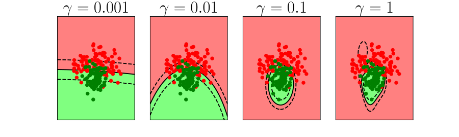
What can these networks represent?

\[ \operatorname{ReLU}(\mathbf{w}_1x - \mathbf{b}_1) \]

What can these networks represent?

\[ f(x) = \mathbf{w}^T_2 \operatorname{ReLU}(\mathbf{w}_1x - \mathbf{b}_1) \]

Single hidden layer

number of kinks \(\approx O(\) width of network \()\)

Example: “sawtooth” network

\[\begin{align} f_l(x) &= 2\vert f_{l-1}(x)\vert - 2 \\ f_0(x) &= x \end{align}\]

Sawtooth network

\[\begin{align} f_l(x) &= 2 \operatorname{ReLU}(f_{l-1}(x)) + 2 \operatorname{ReLU}(-f_{l-1}(x)) - 2\\ f_0(x) &= x \end{align}\]

\(0\)-layer network

\(1\)-layer network

\(2\)-layer network

\(3\)-layer network

\(4\)-layer network

\(5\)-layer network

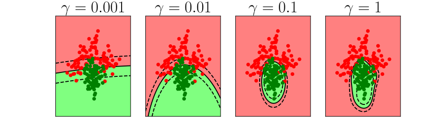
Deep ReLU networks

number of kinks \(\approx O(2^\text{depth of network})\)

In higher dimensions

In higher dimensions

Approximation: summary

• depth increases model complexity more than width
• model clas defined by deep networks is VERY LARGE
• both an advantage, but and cause for concern
• “complex models don’t generalize”

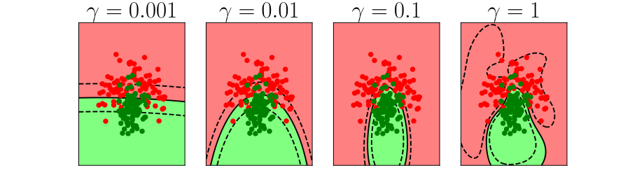
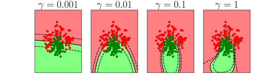
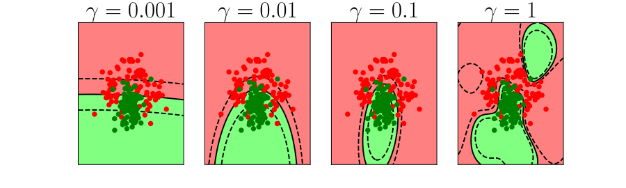
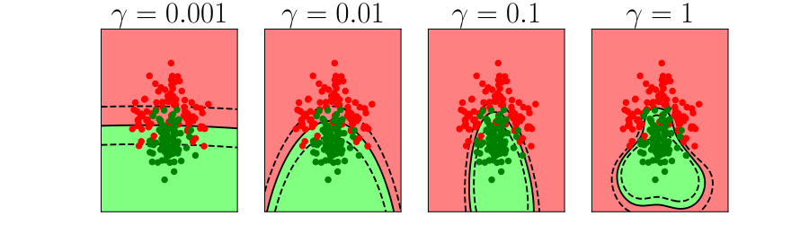
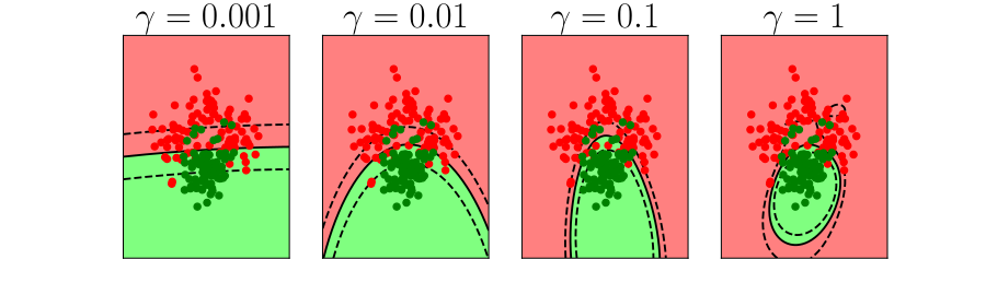
Generalization

Generalization

Generalization

Generalization

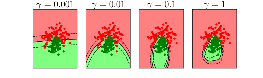
Generalization: deep nets

Generalization: deep nets

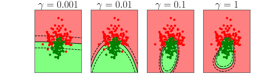
Generalization: summary

• classical view: generalization is property of model class and loss function
• new view: it is also a property of the optimization algorithm

Generalization

• optimization is core to deep learning
• new tools and insights:
  • infinite width neural networks
  • neural tangent kernel (Jacot et al, 2018)
  • deep linear models (e.g. Arora et al, 2019)
  • importance of initialization
  • effect of gradient noise