Visualisation

Visualization and Human Perception

• Human visual system is our highest bandwidth connection to the world
  • Optic tract: ~8.75 million bits/second
  • Verbal communication: only ~2,000 bits/minute
• Active sensing through rapid eye movements (saccades)
  • Not passive reception
  • Actively construct understanding
  • Hundreds of samples per second

Behind the Eye

Visualization and Human Perception

• Visualization is powerful for communication
• But can be vulnerable to manipulation
  • Similar to social media algorithms
  • Misleading visualizations can deceive
  • Can hijack natural visual processing

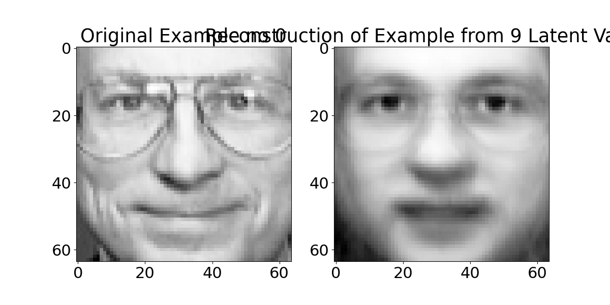
Reconstruction of the Data

Given any posterior projection of a data point, we can replot the original data as a function of the input space.

We will now try to reconstruct the motion capture figure form some different places in the latent plot.

Other Data Sets to Explore

Below there are a few other data sets from pods you might want to explore with PCA. Both of them have \(p\)>\(n\) so you need to consider how to do the larger eigenvalue probleme efficiently without large demands on computer memory.

The data is actually quite high dimensional, and solving the eigenvalue problem in the high dimensional space can take some time. At this point we turn to a neat trick, you don’t have to solve the full eigenvalue problem in the \(p\times p\) covariance, you can choose instead to solve the related eigenvalue problem in the \(n\times n\) space, and in this case \(n=200\) which is much smaller than \(p\).

The original eigenvalue problem has the form \[ \mathbf{Y}^\top\mathbf{Y}\mathbf{U} = \mathbf{U}\boldsymbol{\Lambda} \] But if we premultiply by \(\mathbf{Y}\) then we can solve, \[ \mathbf{Y}\mathbf{Y}^\top\mathbf{Y}\mathbf{U} = \mathbf{Y}\mathbf{U}\boldsymbol{\Lambda} \] but it turns out that we can write \[ \mathbf{U}^\prime = \mathbf{Y}\mathbf{U} \Lambda^{\frac{1}{2}} \] where \(\mathbf{U}^\prime\) is an orthorormal matrix because \[ \left.\mathbf{U}^\prime\right.^\top\mathbf{U}^\prime = \Lambda^{-\frac{1}{2}}\mathbf{U}\mathbf{Y}^\top\mathbf{Y}\mathbf{U} \Lambda^{-\frac{1}{2}} \] and since \(\mathbf{U}\) diagonalises \(\mathbf{Y}^\top\mathbf{Y}\), \[ \mathbf{U}\mathbf{Y}^\top\mathbf{Y}\mathbf{U} = \Lambda \] then \[ \left.\mathbf{U}^\prime\right.^\top\mathbf{U}^\prime = \mathbf{I} \]

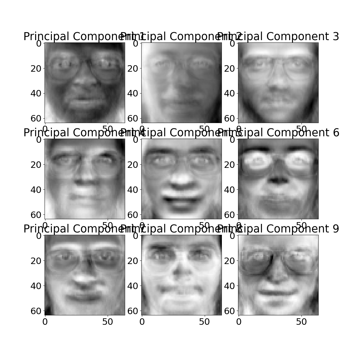
Olivetti Faces

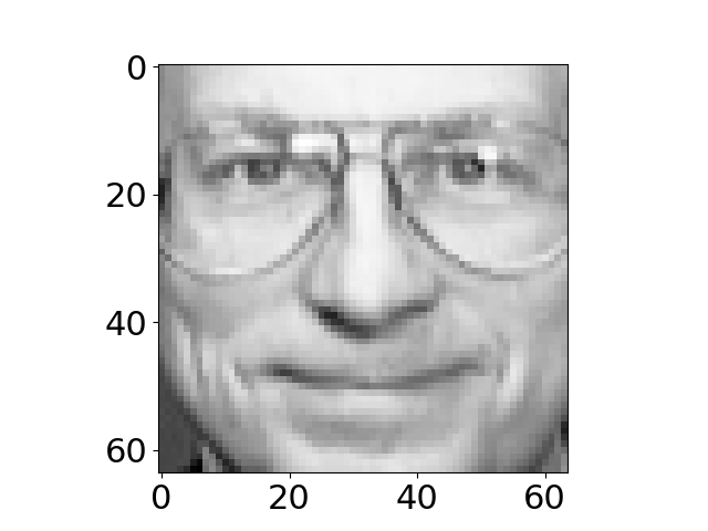
im = np.reshape(Y[1, :].flatten(), (64, 64)).T}

Visualizing the Eigenvectors

Reconstruction

Gene Expression

Multi-Dimensional Scaling

The MDS Objective

Properties of the Frobenius Norm

MDS Solution

Rank-Constrained Solution

Equivalence between MDS and PCA

Connecting the Eigendecompositions

Orthonormalization

Equivalence in Embeddings

Rank-Nullity Connection

Implications

Iterative Dimensionality Reduction

• Spectral methods (PCA, MDS) give analytical solutions
• Iterative methods optimize objective functions
  • Can capture more complex relationships
  • May find local optima
  • More computationally intensive

Stress Functions

Local vs Global Structure Preservation

t-SNE

• Converts distances to probabilities
• Uses t-distribution in low-dimensional space
• Excellent for visualization
• Computationally intensive
• Results depend on perplexity parameter

Oil Flow Data

t-SNE Embedding of Oil Flow Data

UMAP

• Based on Riemannian geometry and algebraic topology
• Preserves both local and global structure
• Faster than t-SNE
• Can be used for general dimension reduction
• Supports supervised and semi-supervised learning

UMAP Parameters

Comparing Dimensionality Reduction Methods

• PCA: Linear, fast, interpretable
• MDS: Distance-based, can be non-linear
• t-SNE: Excellent visualization, local structure
• UMAP: Fast, preserves global structure, versatile